Jones Pupil Analysis

This example demonstrates how to perform a Jones pupil analysis in Optiland. The Jones pupil analysis visualizes the spatially resolved Jones matrix elements across the pupil, providing insight into the polarization properties of the optical system.

import matplotlib.pyplot as plt
from optiland.samples.objectives import CookeTriplet
from optiland.analysis import JonesPupil
from optiland.rays import PolarizationState
from optiland.visualization import OpticViewer

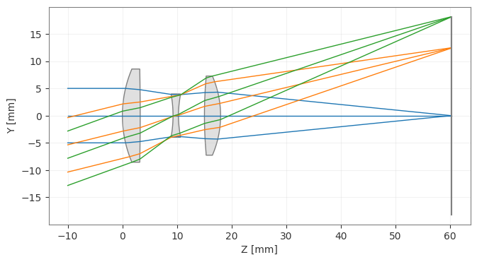
1. Setup the Optical System

We will use a standard Cooke Triplet for this demonstration.

optic = CookeTriplet()

# Set polarization to unpolarized light
state = PolarizationState(is_polarized=False)
optic.updater.set_polarization(state)

# Set Fresnel coatings for all surfaces
optic.surfaces.set_fresnel_coatings()

_ = optic.draw()

2. Basic Jones Pupil Analysis

We instantiate the JonesPupil analysis class with the optic and call the view() method. This generates a grid of plots showing the Real and Imaginary parts of the Jones matrix elements (\(J_{xx}, J_{xy}, J_{yx}, J_{yy}\)) across the pupil.

analysis = JonesPupil(optic)
fig, axs = analysis.view()
plt.show()

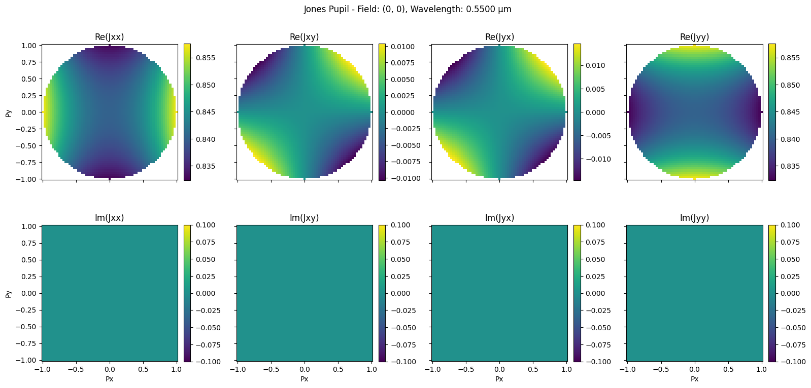
For an on-axis, rotationally symmetric system like the Cooke Triplet, the Jones Pupil reveals geometric polarization aberrations arising from Fresnel effects at curved interfaces.

• Diagonal Terms (:math:`J_{xx}, J_{yy}`): These represent the primary transmission (\(\approx 0.85\)) but display a saddle-like magnitude. This occurs because the transmission for parallel-polarized light (\(T_p\)) is generally higher than for perpendicular-polarized light (\(T_s\)).

  • :math:`J_{xx}`: Maximized along the X-axis (where light is \(p\)-polarized) and minimized along the Y-axis (where light is \(s\)-polarized).

  • :math:`J_{yy}`: Rotated by \(90^\circ\) relative to \(J_{xx}\) (Maximized on Y, minimized on X).

• Off-Diagonal Terms (:math:`J_{xy}, J_{yx}`): These terms represent polarization crosstalk (leakage). They form a characteristic “Maltese Cross” pattern, where leakage is zero along the cardinal axes (\(X, Y\)) and maximizes at the \(\pm 45^\circ\) diagonals due to the geometric rotation of the plane of incidence.

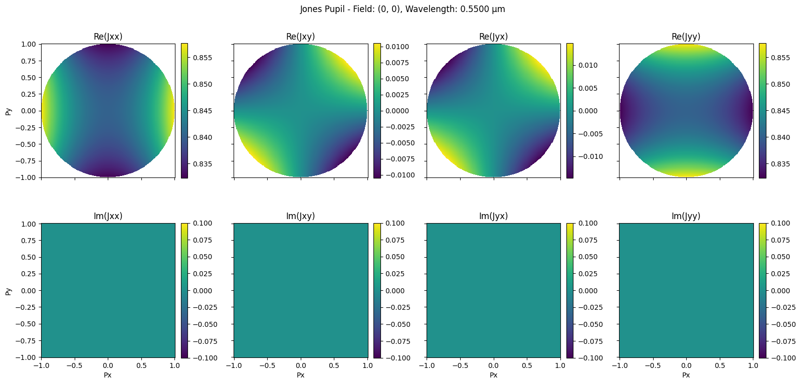
3. Customizing the Analysis

We can customize the analysis by specifying fields, wavelengths, and the grid size.

# Analyze at a specific wavelength and higher resolution
analysis_custom = JonesPupil(optic, wavelengths=[0.55], grid_size=257)
fig, axs = analysis_custom.view()
plt.show()

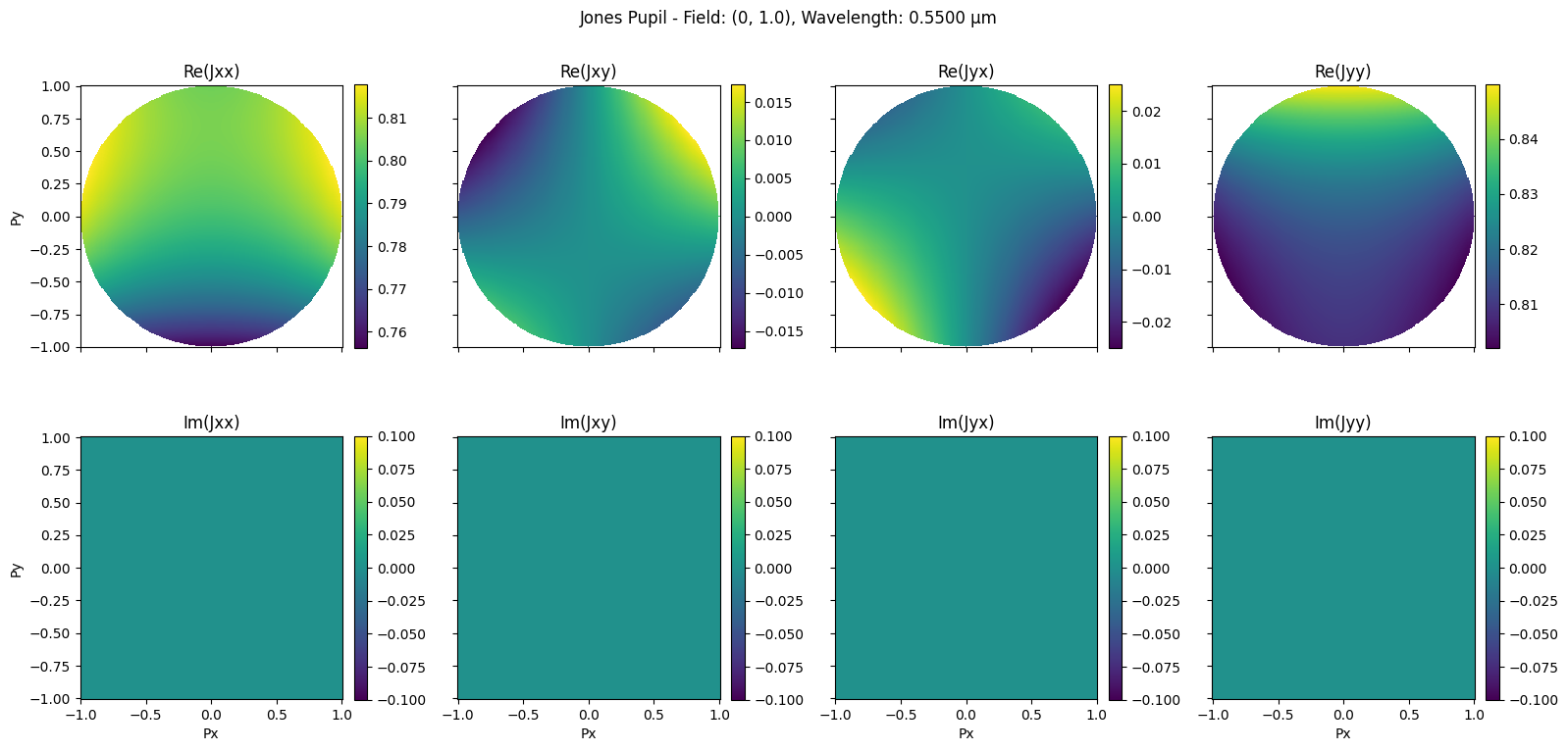
4. Off-Axis Field

Let’s look at an off-axis field point. We first add a field to the optic if it doesn’t exist, or pass it explicitly.

# Passing specific field coordinates (Hx, Hy)
analysis_off_axis = JonesPupil(optic, field=(0, 1.0), grid_size=257)
fig, axs = analysis_off_axis.view()
plt.show()