Image Simulation
This example demonstrates how to simulate the image formation process through an optical system, accounting for:
Spatially Variable Blur: Using EigenPSF decomposition to model PSF variation across the field.
Geometric Distortion: Warping the image based on the lens distortion map.
Lateral Color: Simulating wavelength-dependent magnification/distortion (if multi-wavelength).
We will use the ImageSimulationEngine class.
[1]:
import matplotlib.pyplot as plt
import optiland.backend as be
from optiland.samples.objectives import ReverseTelephoto
from optiland.analysis.image_simulation import ImageSimulationEngine
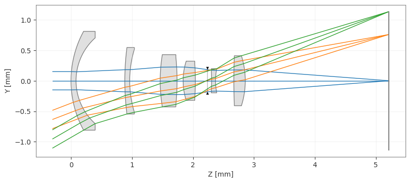
1. Lens Loading
We load a standard ReverseTelephoto lens, which has significant distortion and field-dependent aberrations.
[2]:
optic = ReverseTelephoto()
_ = optic.draw()
2. Select Source Image
Note that the chosen image is based on HopemanMemorialCarillonRecitalSeries2018.jpg by DanielPenfield, used under CC BY-SA 4.0. Simulated images derived from this source are subject to the same license.
[3]:
img_path = 'RushRheesLibrary_800x600.jpg'
3. Run Simulation
We configure the ImageSimulationEngine.
wavelengths: Wavelengths to simulate (RGB).
psf_grid_shape: Number of field points to sample for EigenPSFs (5x5 is usually sufficient).
psf_size: Pixel size of the computed PSFs.
num_rays: Ray density for PSF calculation (higher = more accurate but slower).
[4]:
config = {
    "wavelengths": [0.65, 0.55, 0.45],  # RGB Simulation
    "psf_grid_shape": (5, 5),
    "psf_size": 128,
    "num_rays": 64,
    "oversample": 1
}

simulator = ImageSimulationEngine(optic, config=config)

# Single image input:
# run() accepts an image path, loads it internally, and returns (1, C, H, W).
result = simulator.run(img_path)

print("Output shape:", result.shape)
Output shape: (1, 3, 600, 800)
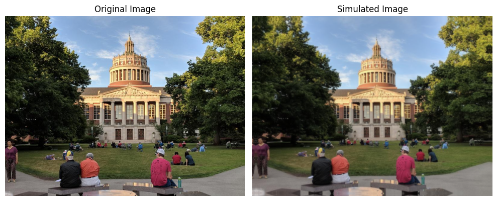
4. View Results
We compare the original and simulated images. A clear blur is visible in the simulated image, indicating the presence of aberrations.
[5]:
_ = simulator.view()
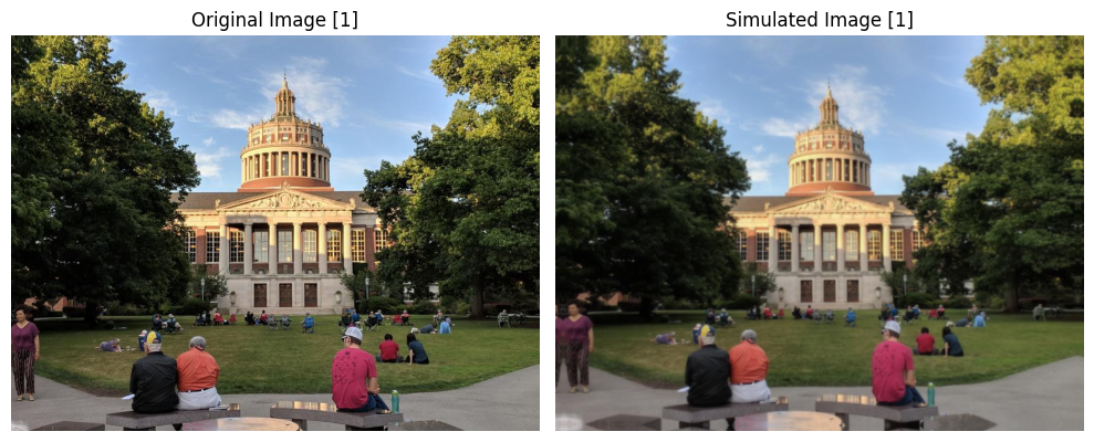
5. Batch Inference
The image simulation engine also supports batched inputs using the (B, C, H, W) format. This is useful for model training or inference workflows where multiple images are processed together.
The view() method can visualize a specific image from the latest batch result using the index argument.
[6]:
# Batched input:
# For batch workflows, pass images directly as (B, C, H, W).
image = plt.imread(img_path)

if image.ndim == 3 and image.shape[-1] == 4:
    image = image[:, :, :3]

image = image.transpose(2, 0, 1)
images = be.array([image, image])

batch_result = simulator.run(images)

print("Batch input shape:", images.shape)
print("Batch output shape:", batch_result.shape)

# Visualize a specific image from the batch
_ = simulator.view(index=1)
Batch input shape: (2, 3, 600, 800)
Batch output shape: (2, 3, 600, 800)
[ ]: