Global Optimization (Differential Evolution)

The following global optimizers are implemented in Optiland: 1. Differential Evolution 2. Dual Annealing 3. SHGO 4. Basin-hopping

These optimizers wrap the scipy.optimize implementations.

import numpy as np

from optiland import optic, optimization

Define a starting lens:

lens = optic.Optic()

# add surfaces
lens.surfaces.add(index=0, radius=np.inf, thickness=np.inf)
lens.surfaces.add(index=1, radius=40, thickness=5, material="SK16", is_stop=True)
lens.surfaces.add(index=2, radius=-100, thickness=50)
lens.surfaces.add(index=3)

# set aperture
lens.set_aperture(aperture_type="EPD", value=20)

# set fields
lens.fields.set_type(field_type="angle")
lens.fields.add(y=0)
lens.fields.add(y=5)

# set wavelength
lens.wavelengths.add(value=0.55, is_primary=True)

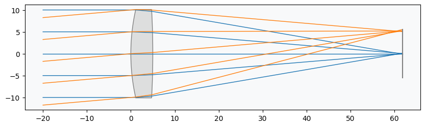
lens.draw()

Define optimization problem:

problem = optimization.OptimizationProblem()

Add operands (targets for optimization):

"""
Add a focal length operand and wavefront error operands for all fields.

Use Gaussian quadrature distribution for the rays (see distribution documentation for
more information).
"""

# focal length target
input_data = {"optic": lens}
problem.add_operand(operand_type="f2", target=60, weight=1, input_data=input_data)

# wavefront error target
for field in lens.fields.get_field_coords():
    input_data = {
        "optic": lens,
        "Hx": field[0],
        "Hy": field[1],
        "num_rays": 3,
        "wavelength": 0.55,
        "distribution": "gaussian_quad",
    }
    problem.add_operand(
        operand_type="OPD_difference",
        target=0,
        weight=1,
        input_data=input_data,
    )

Define variables - let both radii of curvature vary. We will use differential evolution, which requires bounds for all variables.

problem.add_variable(lens, "radius", surface_number=1, min_val=-500, max_val=500)
problem.add_variable(lens, "radius", surface_number=2, min_val=-500, max_val=500)

Let thicknesses to image plane vary:

problem.add_variable(lens, "thickness", surface_number=2, min_val=30, max_val=100)

Check initial merit function value and system properties:

problem.info()

╒════╤════════════════════════╤═══════════════════╕
│    │   Merit Function Value │   Improvement (%) │
╞════╪════════════════════════╪═══════════════════╡
│  0 │                3716.81 │                 0 │
╘════╧════════════════════════╧═══════════════════╛
╒════╤════════════════╤══════════╤══════════╤═════════╤══════════╤════════════════════╕
│    │ Operand Type   │   Target │   Weight │   Value │    Delta │   Contribution (%) │
╞════╪════════════════╪══════════╪══════════╪═════════╪══════════╪════════════════════╡
│  0 │ f2             │       60 │        1 │ 46.5275 │ -13.4725 │            4.88345 │
│  1 │ OPD difference │        0 │        1 │ 56.0052 │  56.0052 │           84.3891  │
│  2 │ OPD difference │        0 │        1 │ 19.968  │  19.968  │           10.7275  │
╘════╧════════════════╧══════════╧══════════╧═════════╧══════════╧════════════════════╛
╒════╤═════════════════╤═══════════╤═════════╤══════════════╤══════════════╕
│    │ Variable Type   │   Surface │   Value │   Min. Bound │   Max. Bound │
╞════╪═════════════════╪═══════════╪═════════╪══════════════╪══════════════╡
│  0 │ radius          │         1 │      40 │         -500 │          500 │
│  1 │ radius          │         2 │    -100 │         -500 │          500 │
│  2 │ thickness       │         2 │      50 │           30 │          100 │
╘════╧═════════════════╧═══════════╧═════════╧══════════════╧══════════════╛

Define optimizer:

optimizer = optimization.DifferentialEvolution(problem)

Run optimization:

# workers=-1 uses all available cores
optimizer.optimize(maxiter=256, disp=False, workers=-1)

             message: Optimization terminated successfully.
             success: True
                 fun: 3.612745542781897
                   x: [-5.386e-01 -2.897e+00  4.682e+00]
                 nit: 69
                nfev: 3462
          population: [[-5.386e-01 -2.897e+00  4.682e+00]
                       [-5.320e-01 -2.821e+00  4.705e+00]
                       ...
                       [-5.352e-01 -2.862e+00  4.696e+00]
                       [-5.356e-01 -2.837e+00  4.676e+00]]
 population_energies: [ 3.613e+00  3.772e+00 ...  3.656e+00  3.675e+00]
                 jac: [ 1.009e+03  2.971e+01  4.932e+01]

Print merit function value and system properties after optimization:

problem.info()

╒════╤════════════════════════╤═══════════════════╕
│    │   Merit Function Value │   Improvement (%) │
╞════╪════════════════════════╪═══════════════════╡
│  0 │                3.61275 │           99.9028 │
╘════╧════════════════════════╧═══════════════════╛
╒════╤════════════════╤══════════╤══════════╤══════════╤══════════╤════════════════════╕
│    │ Operand Type   │   Target │   Weight │    Value │    Delta │   Contribution (%) │
╞════╪════════════════╪══════════╪══════════╪══════════╪══════════╪════════════════════╡
│  0 │ f2             │       60 │        1 │ 60.1043  │ 0.104299 │           0.301108 │
│  1 │ OPD difference │        0 │        1 │  1.30422 │ 1.30422  │          47.0832   │
│  2 │ OPD difference │        0 │        1 │  1.37872 │ 1.37872  │          52.6157   │
╘════╧════════════════╧══════════╧══════════╧══════════╧══════════╧════════════════════╛
╒════╤═════════════════╤═══════════╤═══════════╤══════════════╤══════════════╕
│    │ Variable Type   │   Surface │     Value │   Min. Bound │   Max. Bound │
╞════╪═════════════════╪═══════════╪═══════════╪══════════════╪══════════════╡
│  0 │ radius          │         1 │   46.1442 │         -500 │          500 │
│  1 │ radius          │         2 │ -189.732  │         -500 │          500 │
│  2 │ thickness       │         2 │   56.8164 │           30 │          100 │
╘════╧═════════════════╧═══════════╧═══════════╧══════════════╧══════════════╛

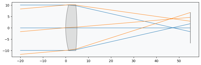
Draw final lens:

lens.draw(num_rays=5)