Tutorial 4c - Zernike Decomposition

This tutorial shows how to decompose the pupil using various Zernike types. Namely, we use “standard”, “fringe”, and “Noll” Zernike indices.

import matplotlib.pyplot as plt

from optiland import wavefront
from optiland.samples.eyepieces import EyepieceErfle

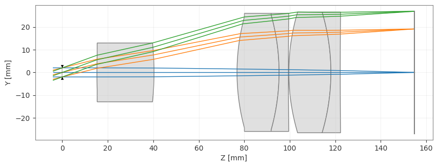
lens = EyepieceErfle()
lens.draw()

(<Figure size 1000x400 with 1 Axes>, <Axes: xlabel='Z [mm]', ylabel='Y [mm]'>)

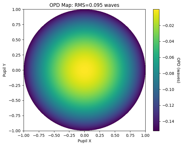
First, we’ll view the wavefront.

opd = wavefront.OPD(lens, field=(0, 0), wavelength=0.55)
opd.view(projection="2d", num_points=512)

(<Figure size 700x550 with 2 Axes>,
 <Axes: title={'center': 'OPD Map: RMS=0.095 waves'}, xlabel='Pupil X', ylabel='Pupil Y'>)

We’ll then find the Zernike coefficients of the wavefront.

zernike_standard = wavefront.ZernikeOPD(
    lens,
    field=(0, 0),
    wavelength=0.55,
    zernike_type="standard",
    num_terms=37,
)

Let’s view the Zernike fit and compare it to the nominal OPD map.

zernike_standard.view(projection="2d", num_points=512)

(<Figure size 700x550 with 2 Axes>,
 <Axes: title={'center': 'Zernike Standard Fit'}, xlabel='Pupil X', ylabel='Pupil Y'>)

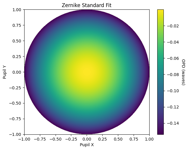
Qualitatively, we can see the Zernike fit well-represents the OPD map.

Let’s see what the actual coefficients look like:

plt.bar(range(1, 38), zernike_standard.coeffs)
plt.axhline(color="k", linewidth=1, linestyle="--")
plt.xlabel("Zernike Term #")
plt.ylabel("Zernike Standard Coefficient")
plt.show()

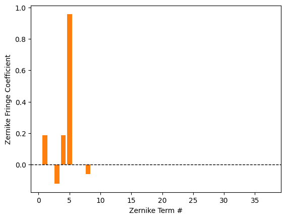
Let’s decompose the wavefront using Zernike fringe indices and Zernike Noll indices. We’ll use the field point at (0, 1).

zernike_fringe = wavefront.ZernikeOPD(
    lens,
    field=(0, 1),
    wavelength=0.55,
    zernike_type="fringe",
    num_terms=37,
)

plt.bar(range(1, 38), zernike_fringe.coeffs, color="C1")
plt.axhline(color="k", linewidth=1, linestyle="--")
plt.xlabel("Zernike Term #")
plt.ylabel("Zernike Fringe Coefficient")
plt.show()

zernike_noll = wavefront.ZernikeOPD(
    lens,
    field=(0, 1),
    wavelength=0.55,
    zernike_type="noll",
    num_terms=37,
)

plt.bar(range(1, 38), zernike_noll.coeffs, color="C2")
plt.axhline(color="k", linewidth=1, linestyle="--")
plt.xlabel("Zernike Term #")
plt.ylabel("Zernike Noll Coefficient")
plt.show()

Or, if we just want to read off the coefficients, we can print them. Let’s only use 9 terms in this case:

zernike = wavefront.ZernikeOPD(lens, (0, 1), 0.55, zernike_type="noll", num_terms=9)

for k in range(len(zernike.coeffs)):
    print(f"Z{k + 1}: {zernike.coeffs[k]:.8f}")

Z1: 0.18585891
Z2: -0.00000000
Z3: -0.06086925
Z4: 0.10781267
Z5: 0.00000000
Z6: 0.39115859
Z7: -0.02152073
Z8: -0.00000000
Z9: 0.00002531