Tutorial 4b - PSF and MTF Calculation
This tutorial shows how to calculate the point spread function (PSF) and modulation transfer function (MTF) of a lens.
[1]:
from optiland import mtf, psf
from optiland.samples.objectives import CookeTriplet
[2]:
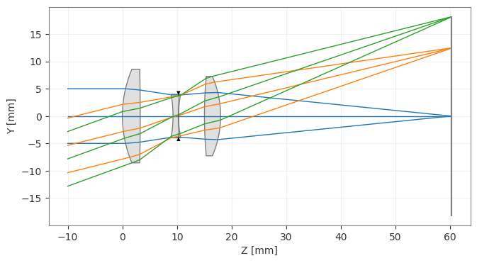
lens = CookeTriplet()
lens.draw()
[2]:
(<Figure size 1000x400 with 1 Axes>, <Axes: xlabel='Z [mm]', ylabel='Y [mm]'>)
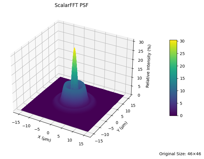
We first compute the PSF using the FFT-based approach. We demonstrate various ways to generate and plot the PSF.
[3]:
lens_psf = psf.FFTPSF(lens, field=(0, 0), wavelength=0.55)
lens_psf.view(projection="3d", num_points=256)
C:\Users\kdani\AppData\Local\Temp\ipykernel_30580\3512864652.py:2: UserWarning: The PSF view has a high oversampling factor (5.57). Results may be inaccurate.
  lens_psf.view(projection="3d", num_points=256)
[3]:
(<Figure size 700x550 with 2 Axes>,
 <Axes3D: title={'center': 'ScalarFFT PSF'}, xlabel='X (µm)', ylabel='Y (µm)', zlabel='Relative Intensity (%)'>)
[4]:
print(f"Strehl Ratio: {lens_psf.strehl_ratio():.3f}")
Strehl Ratio: 0.306
[5]:
lens_psf = psf.FFTPSF(lens, field=(0, 0.7), wavelength=0.55)
lens_psf.view(num_points=512)
C:\Users\kdani\AppData\Local\Temp\ipykernel_30580\3051880103.py:2: UserWarning: The PSF view has a high oversampling factor (4.65). Results may be inaccurate.
  lens_psf.view(num_points=512)
[5]:
(<Figure size 700x550 with 2 Axes>,
 <Axes: title={'center': 'ScalarFFT PSF'}, xlabel='X (µm)', ylabel='Y (µm)'>)
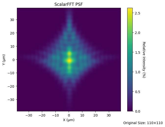
[6]:
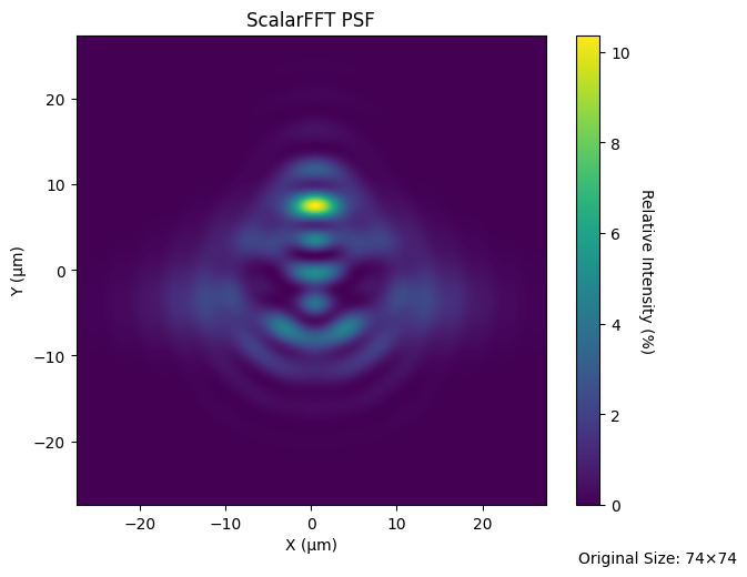
lens_psf = psf.FFTPSF(lens, field=(0, 1.0), wavelength=0.55)
lens_psf.view(projection="2d", num_points=256)
C:\Users\kdani\AppData\Local\Temp\ipykernel_30580\48181633.py:2: UserWarning: The PSF view has a high oversampling factor (3.46). Results may be inaccurate.
  lens_psf.view(projection="2d", num_points=256)
[6]:
(<Figure size 700x550 with 2 Axes>,
 <Axes: title={'center': 'ScalarFFT PSF'}, xlabel='X (µm)', ylabel='Y (µm)'>)
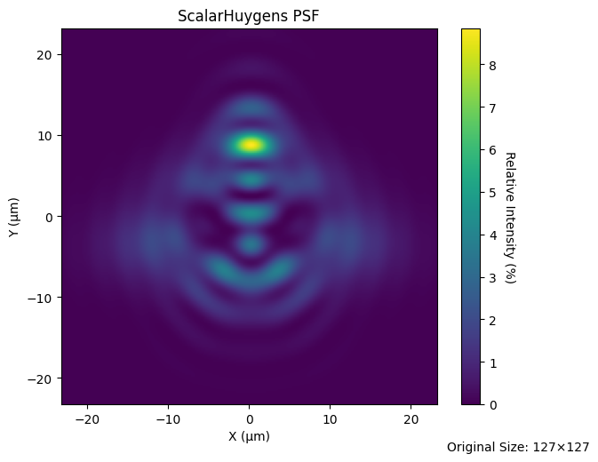
We can also generate the PSF using direct Huygens-Fresnel integration. This is referred to as the “Huygens PSF”.
[7]:
lens_huygens_psf = psf.HuygensPSF(lens, field=(0, 1.0), wavelength=0.55)
lens_huygens_psf.view(projection="2d", num_points=256)
[7]:
(<Figure size 700x550 with 2 Axes>,
 <Axes: title={'center': 'ScalarHuygens PSF'}, xlabel='X (µm)', ylabel='Y (µm)'>)
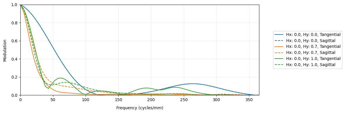
Now, we generate the geometric MTF, which uses only ray intersection locations on the image plane and ignores diffraction. The geometric MTF is a reasonable approximation when the lens is far from the diffraction limit.
As is standard, the geometric MTF is scaled based on the diffraction-limited MTF curve. This assures that the geometric MTF cannot show performance better than the diffraction limit.
[8]:
geo_mtf = mtf.GeometricMTF(lens)
geo_mtf.view()
[8]:
(<Figure size 1200x400 with 1 Axes>,
 <Axes: xlabel='Frequency (cycles/mm)', ylabel='Modulation'>)
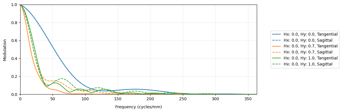
Finally, we show the standard FFT-based MTF.
[9]:
lens_mtf = mtf.FFTMTF(lens)
lens_mtf.view()
[9]:
(<Figure size 1200x400 with 1 Axes>,
 <Axes: xlabel='Frequency (cycles/mm)', ylabel='Modulation'>)