Tutorial 2a - Tracing and Analyzing Rays
The 2D visualization is now interactive! You can hover over surfaces, lenses, and ray bundles to get more information. You can also customize the look and feel of the plots using themes. See the gallery for an example of how to use themes.
This tutorial shows how to trace rays through a system, and how ray information can be retrieved and analyzed.
[1]:
import matplotlib.pyplot as plt

from optiland import distribution
from optiland.samples.objectives import ReverseTelephoto
[2]:
lens = ReverseTelephoto()
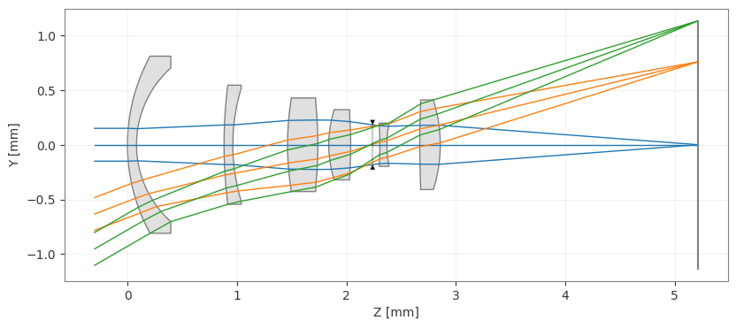
[3]:
lens.draw()
[3]:
(<Figure size 1000x400 with 1 Axes>, <Axes: xlabel='Z [mm]', ylabel='Y [mm]'>)
First, we’ll take a look at a few different pupil grids that we can trace through the system. Note that each distribution has x and y attributes, which are NumPy arrays containing the points of the distribution.
[4]:
dist_rand = distribution.RandomDistribution(seed=None)
dist_rand.generate_points(num_points=100)
dist_rand.view()
[4]:
(<Figure size 640x480 with 1 Axes>,
 <Axes: xlabel='Normalized Pupil Coordinate X', ylabel='Normalized Pupil Coordinate Y'>)
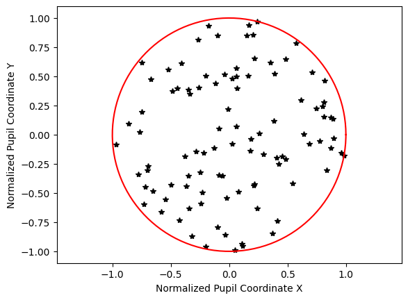
Note that for a uniform distribution, we define the number of points along one axis.
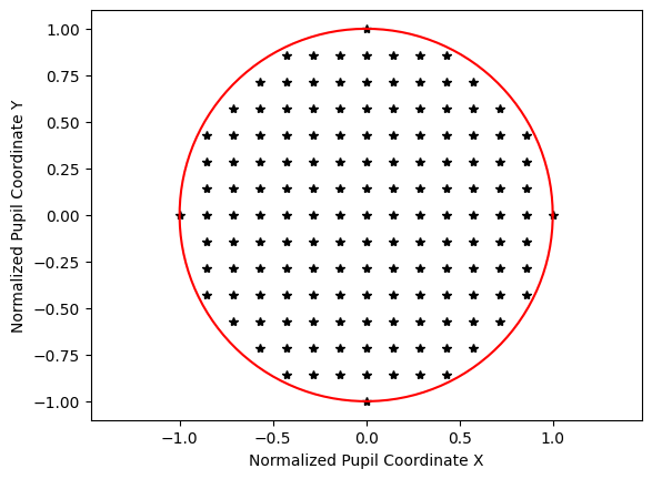
[5]:
dist_uniform = distribution.UniformDistribution()
dist_uniform.generate_points(num_points=15)
dist_uniform.view()
[5]:
(<Figure size 640x480 with 1 Axes>,
 <Axes: xlabel='Normalized Pupil Coordinate X', ylabel='Normalized Pupil Coordinate Y'>)
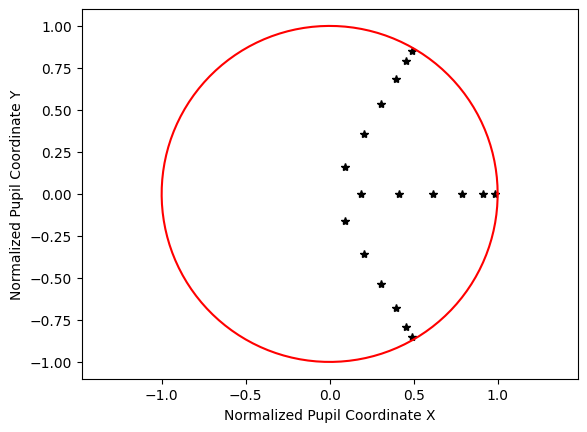
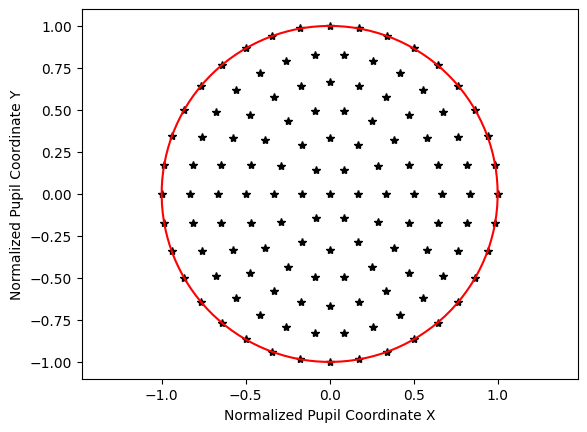
The next distribution is the Gaussian qaudrature, which is an optimized grid for lens design based on the following paper. Essentially, this grid probes the pupil in such a way so as to accurately determine the wavefront while minimizing the number of rays traced.
Forbes, “Optical system assessment for design: numerical ray tracing in the Gaussian pupil,” J. Opt. Soc. Am. A 5, 1943-1956 (1988)
[6]:
dist_quad = distribution.GaussianQuadrature(is_symmetric=False)
dist_quad.generate_points(num_rings=6)
dist_quad.view()
[6]:
(<Figure size 640x480 with 1 Axes>,
 <Axes: xlabel='Normalized Pupil Coordinate X', ylabel='Normalized Pupil Coordinate Y'>)
[7]:
dist_hex = distribution.HexagonalDistribution()
dist_hex.generate_points(num_rings=6)
dist_hex.view()
[7]:
(<Figure size 640x480 with 1 Axes>,
 <Axes: xlabel='Normalized Pupil Coordinate X', ylabel='Normalized Pupil Coordinate Y'>)
Now, let’s trace a grid of rays through the reverse telephoto lens.
We use the normalized field coordinates (Hx, Hy) and trace the on-axis field at (0, 0). We specify the wavelength and grid distribution.
[8]:
rays = lens.trace(Hx=0, Hy=0, wavelength=0.55, num_rays=1024, distribution="random")
There are many ray properties we can extract:
x, y, z intersections per surface
L, M, N ray direction cosines per surface
Ray intensity
Ray optical path length
Let’s plot a few of these to show how to access them.
[9]:
num_surfaces = lens.surfaces.num_surfaces

# take intersection points on last surface only
x_image = lens.surfaces.x[num_surfaces - 1, :]
y_image = lens.surfaces.y[num_surfaces - 1, :]
[10]:
plt.scatter(x_image, y_image, s=3)
plt.axis("image")
plt.xlabel("X [mm]")
plt.ylabel("Y [mm]")
plt.title("Field Point (0, 0), $\\lambda$=0.55 µm")
plt.show()

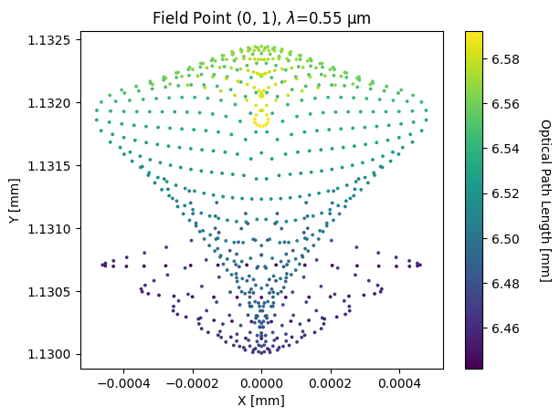
Let’s add the optical path length of the ray as the color attribute of each point. Let’s trace a different distribution to use for plotting.
[11]:
lens.trace(Hx=0, Hy=1, wavelength=0.55, num_rays=15, distribution="hexapolar")
[11]:
<optiland.rays.real_rays.RealRays at 0x23bd410ff50>
[12]:
opd = lens.surfaces.opd[num_surfaces - 1, :]
x_image = lens.surfaces.x[num_surfaces - 1, :]
y_image = lens.surfaces.y[num_surfaces - 1, :]

plt.scatter(x_image, y_image, s=3, c=opd)
plt.xlabel("X [mm]")
plt.ylabel("Y [mm]")
plt.title("Field Point (0, 1), $\\lambda$=0.55 µm")
cbar = plt.colorbar()
cbar.ax.get_yaxis().labelpad = 25
cbar.ax.set_ylabel("Optical Path Length [mm]", rotation=270)
plt.show()
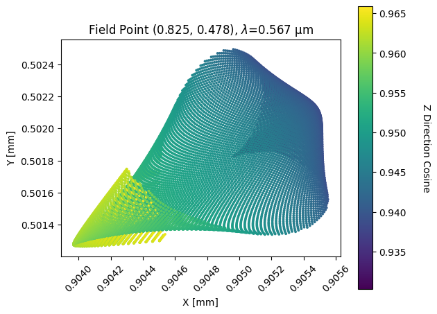
Lastly, let’s look at the z direction cosine of the rays. This shows how close the rays are to parallel with the optical axis.
Again, let’s retrace a grid of rays. This time we’ll use an arbitrary field with “many” rays (≈128**2)
[13]:
rays = lens.trace(
    Hx=0.825,
    Hy=0.478,
    wavelength=0.567,
    num_rays=128,
    distribution="uniform",
)
[14]:
x_image = lens.surfaces.x[num_surfaces - 1, :]
y_image = lens.surfaces.y[num_surfaces - 1, :]
N = lens.surfaces.N[num_surfaces - 1, :]

plt.scatter(x_image, y_image, s=3, c=N)
plt.axis("image")
plt.xlabel("X [mm]")
plt.ylabel("Y [mm]")
plt.title("Field Point (0.825, 0.478), $\\lambda$=0.567 µm")
cbar = plt.colorbar()
cbar.ax.get_yaxis().labelpad = 25
cbar.ax.set_ylabel("Z Direction Cosine", rotation=270)
plt.xticks(rotation=45)
plt.tight_layout()
plt.show()
There are many other properties available, which can be seen in optiland.surfaces.SurfaceGroup.
In general, the ray information is saved in a 2D matrix with shape (num_surfaces x num_rays). All ray information is available after ray tracing, which can be configured generically. For example, various distributions can be used, but user-defined rays may also be specified. This will be discussed later.