Derivation of the Statistical Dispersion Model for Optiland’s AbbeMaterial - 2026 Update
Kramer Harrison, 2026
1. Introduction
In first-order optical design, materials are often defined solely by their refractive index (\(n_d\)) and Abbe number (\(V_d\)). While sufficient for paraxial achromatization, this two-parameter definition is mathematically under-determined: infinite dispersion curves can satisfy a single (\(n_d, V_d\)) pair.
Standard approximations, such as the “Normal Line” rule, assume a fixed linear relationship between partial dispersion (\(P_{g,F}\)) and Abbe number. While effective for standard crowns and flints, this heuristic fails for “anomalous” glasses (e.g., fluor-crowns or dense flints), leading to significant index prediction errors in the deep blue (\(<0.45 \mu m\)) and near-infrared.
Objective
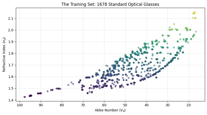
This study derives a robust, data-driven dispersion model to resolve this ambiguity. By analyzing refractive index data of over 1,000 commercial optical glasses, we aim to:
Determine Dimensionality: Use Principal Component Analysis (PCA) to quantify the effective degrees of freedom in standard optical glasses.
Select a Basis: Apply LassoLarsIC (Sparse Regression) to the Buchdahl dispersion formula to identify the minimum set of coefficients required for accurate spectral reconstruction.
Validate Stability: Demonstrate that this sparse, physics-informed model minimizes spectral error compared to standard linear approximations.
[1]:
import warnings
import pandas as pd
import numpy as np
import os
import matplotlib.pyplot as plt
from sklearn.decomposition import PCA
from sklearn.linear_model import LassoLarsIC, LinearRegression
from sklearn.pipeline import make_pipeline
from sklearn.preprocessing import StandardScaler
from scipy.optimize import curve_fit
from optiland.materials import MaterialFile
[2]:
# Configuration
CATALOG_PATH = '../../database/catalog_nk.csv'  # in Optiland's database dir
DATA_DIR = '../../database/data-nk/'  # in Optiland's database dir

# We filter for established manufacturers to ensure we are modeling
# the physics of stable, amorphous silicate/phosphate glasses.
VALID_CATALOGS = [
    'schott', 'ohara', 'hoya', 'cdgm', 'sumita', 'hikari'
]

# Wavelength grid for analysis (Extended Visible: 0.38 - 0.78 µm)
WAVE_GRID = np.linspace(0.380, 0.780, 100)
[3]:
# Define standard reference wavelengths for Abbe definition
# Helium d-line (yellow), Hydrogen F (blue), Hydrogen C (red)
WAVE_D = 0.5875618
WAVE_F = 0.4861327
WAVE_C = 0.6562725

def load_standard_glasses(catalog_path=CATALOG_PATH, wave_grid=WAVE_GRID):
    """
    Ingests the glass database and filters for physically standard optical glasses.
    Returns a DataFrame containing the 'Ground Truth' dispersion curves.
    """
    print(f"Loading glass database from {catalog_path}...")

    if not os.path.exists(catalog_path):
        raise FileNotFoundError(f"Catalog file not found at: {catalog_path}")

    df_raw = pd.read_csv(catalog_path)
    valid_data = []

    # Statistics for the log
    stats = {'total': len(df_raw), 'success': 0, 'range_skip': 0, 'error_skip': 0, 'manuf_skip': 0}

    # Standard glass range settings
    ND_MIN, ND_MAX = 1.35, 2.6
    VD_MIN, VD_MAX = 15.0, 100.0

    for idx, row in df_raw.iterrows():
        # 1. Manufacturer Check
        f_name = str(row.get('filename', '')).lower()
        g_name = str(row.get('group', '')).lower()
        identifier = f_name + g_name

        is_valid_catalog = any(c in identifier for c in VALID_CATALOGS)

        if not is_valid_catalog:
            stats['manuf_skip'] += 1
            continue

        filepath = os.path.join(DATA_DIR, row['filename'])
        if not os.path.exists(filepath):
            stats['error_skip'] += 1
            continue

        try:
            # 2. Load material
            with warnings.catch_warnings():
                warnings.simplefilter("ignore")
                mat = MaterialFile(filepath)

                # Abbe Definitions
                nd = mat.n(WAVE_D).item()
                nF = mat.n(WAVE_F).item()
                nC = mat.n(WAVE_C).item()

            # 3. Physics & Range Sanity Checks
            if np.isnan(nd) or nd <= 1.0:
                stats['error_skip'] += 1
                continue

            dispersion = nF - nC
            if dispersion <= 1e-9:
                stats['error_skip'] += 1
                continue

            Vd = (nd - 1) / dispersion

            # Filter out extreme materials
            if not (ND_MIN < nd < ND_MAX):
                stats['range_skip'] += 1
                continue

            if not (VD_MIN < Vd < VD_MAX):
                stats['range_skip'] += 1
                continue

            # 4. Generate full spectral curve
            with warnings.catch_warnings():
                warnings.simplefilter("ignore")
                curve = mat.n(wave_grid)

            if np.any(np.isnan(curve)):
                stats['error_skip'] += 1
                continue

            valid_data.append({
                'name': row['name'],
                'nd': nd,
                'Vd': Vd,
                'curve': curve
            })
            stats['success'] += 1

        except Exception:
            stats['error_skip'] += 1
            continue

    df = pd.DataFrame(valid_data)

    print("-" * 60)
    print(f"Data Ingestion Complete.")
    print(f"Total entries: {stats['total']}")
    print(f"Successfully loaded: {stats['success']}")
    print(f"Skipped (Manufacturer): {stats['manuf_skip']}")
    print(f"Skipped (Out of Range): {stats['range_skip']}")
    print("-" * 60)

    return df
[4]:
# Execute data loading
df_glass = load_standard_glasses(CATALOG_PATH, WAVE_GRID)
Loading glass database from ../../database/catalog_nk.csv...
------------------------------------------------------------
Data Ingestion Complete.
Total entries: 3201
Successfully loaded: 1678
Skipped (Manufacturer): 1516
Skipped (Out of Range): 6
------------------------------------------------------------
[5]:
# Visualization: Glass diagram for dataset
plt.figure(figsize=(10, 5))
plt.scatter(
    df_glass['Vd'],
    df_glass['nd'],
    c=df_glass['nd'],
    cmap='viridis',
    s=25,
    alpha=0.6,
    edgecolors='k',
    linewidth=0.2
)
plt.gca().invert_xaxis()
plt.title(f"The Training Set: {len(df_glass)} Standard Optical Glasses")
plt.xlabel("Abbe Number ($V_d$)")
plt.ylabel("Refractive Index ($n_d$)")
plt.grid(True, alpha=0.3)
plt.show()
2. Determining the Optimal Basis Function
To construct a model, we must first choose a mathematical basis function \(f(\lambda)\). While polynomials (\(A + B\lambda + C\lambda^2\)) or Cauchy equations are common, they may not be the most efficient representation for typical glass dispersion.
We apply Principal Component Analysis (PCA) to the dataset to determine the effective dimensionality of the problem and identifying the optimal functional shape. We subtract the base refractive index (\(n_d\)) from each curve to isolate the dispersion shape.
Hypothesis
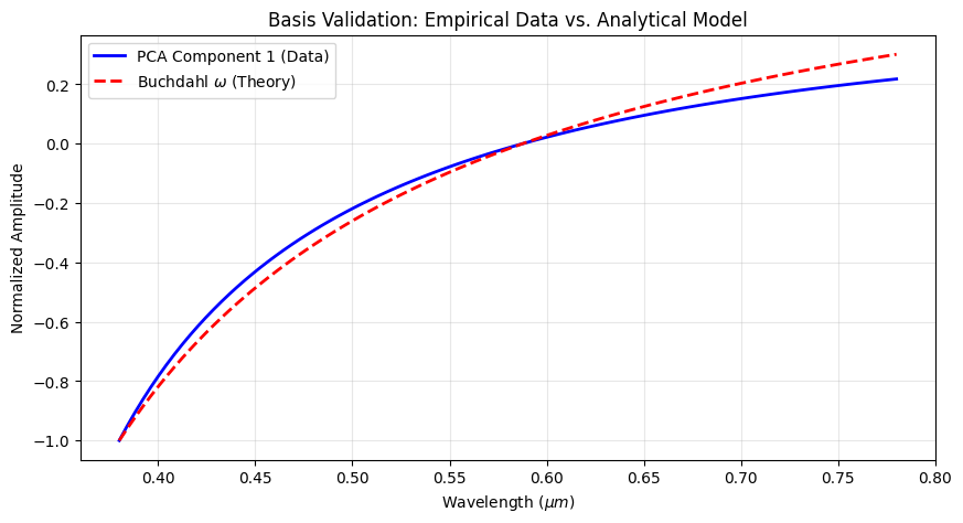
The Buchdahl dispersion model utilizes a coordinate transformation \(\omega\) designed to linearize the dispersion of silicate glasses:
If this coordinate transformation is physically robust, the first principal component (PC1) of our data should strongly correlate with \(\omega\).
[6]:
# Constants
LAM_D = 0.5875618

def buchdahl_coordinate(lam):
    """
    Transforms wavelength to the normalized Buchdahl coordinate.
    """
    return (lam - LAM_D) / (1.0 + 2.5 * (lam - LAM_D))
[7]:
# --- PCA Execution ---
# 1. Prepare Data Matrix
# Shape: (n_samples, n_wavelengths)
X_curves = np.vstack(df_glass['curve'].values)

# 2. Center the data per-sample
# We subtract nd to focus purely on the dispersion slope and curvature,
# removing the "piston" term (absolute index).
nd_vector = df_glass['nd'].values[:, np.newaxis]
X_dispersion = X_curves - nd_vector

# 3. Fit PCA
pca = PCA(n_components=3)  # choose 3 components
pca.fit(X_dispersion)
[7]:
PCA(n_components=3)In a Jupyter environment, please rerun this cell to show the HTML representation or trust the notebook.
On GitHub, the HTML representation is unable to render, please try loading this page with nbviewer.org.
Parameters
[8]:
# Report Explained Variance
print("--- Effective Degrees of Freedom (Visible Spectrum) ---")
variance = pca.explained_variance_ratio_
print(f"PC1 (Primary Dispersion):   {variance[0]*100:.5f}%")
print(f"PC2 (Secondary Curvature):  {variance[1]*100:.5f}%")
print(f"PC3 (Residuals):            {variance[2]*100:.5f}%")
print(f"Total Explained (3 terms):  {np.sum(variance)*100:.6f}%")
--- Effective Degrees of Freedom (Visible Spectrum) ---
PC1 (Primary Dispersion):   99.91697%
PC2 (Secondary Curvature):  0.08068%
PC3 (Residuals):            0.00226%
Total Explained (3 terms):  99.999913%
As can be seen, 3 components alone account for >99.9999% of the variance in the refractive index data.
[9]:
# --- Visualization: Buchdahl vs. Data ---
w_vec = buchdahl_coordinate(WAVE_GRID)

# Align signs for visual comparison (PCA sign is arbitrary)
pc1 = pca.components_[0]
if np.corrcoef(pc1, w_vec)[0, 1] < 0:
    pc1 = -pc1

# Normalize for plotting shape comparison
pc1_norm = pc1 / np.max(np.abs(pc1))
w_vec_norm = w_vec / np.max(np.abs(w_vec))

plt.figure(figsize=(10, 5))
plt.plot(WAVE_GRID, pc1_norm, 'b-', linewidth=2, label='PCA Component 1 (Data)')
plt.plot(WAVE_GRID, w_vec_norm, 'r--', linewidth=2, label=r'Buchdahl $\omega$ (Theory)')
plt.title("Basis Validation: Empirical Data vs. Analytical Model")
plt.xlabel(r"Wavelength ($\mu m$)")
plt.ylabel("Normalized Amplitude")
plt.legend()
plt.grid(True, alpha=0.3)
plt.show()
3. Analyzing the Coefficients
Having validated that the Buchdahl coordinate is a suitable proxy for the primary dispersion vector, we adopt the 3-term Buchdahl model:
We fit this equation to every glass in the dataset to extract the “True” coefficients. This allows us to inspect how these coefficients relate to the input parameters (\(n_d, V_d\)).
The “Partial Dispersion” Problem
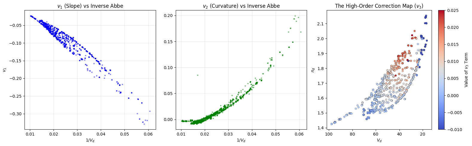
Standard 2-parameter models typically assume: 1. \(v_1\) is linear with \(1/V_d\). 2. \(v_2\) is linear with \(1/V_d\). 3. \(v_3\) is zero.
We visualize the calculated \(v_3\) term on the Abbe diagram. A non-random pattern would indicate that \(v_3\) is not noise, but a systematic property of the glass chemistry that we can predict.
[10]:
def buchdahl_3term(w, v1, v2, v3, nd_fixed):
    """
    3-term Buchdahl model with fixed intercept.
    """
    return nd_fixed + v1 * w + v2 * (w**2) + v3 * (w**3)
[11]:
# --- Extract Coefficients ---
results = []
w_grid_calc = buchdahl_coordinate(WAVE_GRID)

print("Extracting coefficients for all glasses...")

for idx, row in df_glass.iterrows():
    # Define objective function for this specific glass
    nd_glass = row['nd']

    def objective(w, v1, v2, v3):
        return buchdahl_3term(w, v1, v2, v3, nd_glass)

    try:
        # Initial guess [0,0,0] is important for convergence stability
        popt, _ = curve_fit(objective, w_grid_calc, row['curve'], p0=[0, 0, 0])

        results.append({
            'nd': row['nd'],
            'Vd': row['Vd'],
            'v1': popt[0],
            'v2': popt[1],
            'v3': popt[2]
        })
    except Exception:
        continue

df_coeffs = pd.DataFrame(results)
Extracting coefficients for all glasses...
[12]:
# --- Visualization ---
fig, axes = plt.subplots(1, 3, figsize=(16, 5))

# Plot 1: v1 vs 1/Vd (Check Linearity)
axes[0].scatter(1.0/df_coeffs['Vd'], df_coeffs['v1'], s=5, alpha=0.4, c='blue')
axes[0].set_title("$v_1$ (Slope) vs Inverse Abbe")
axes[0].set_xlabel("$1/V_d$")
axes[0].set_ylabel("$v_1$")
axes[0].grid(True, alpha=0.3)

# Plot 2: v2 vs 1/Vd (Check Curvature)
axes[1].scatter(1.0/df_coeffs['Vd'], df_coeffs['v2'], s=5, alpha=0.4, c='green')
axes[1].set_title("$v_2$ (Curvature) vs Inverse Abbe")
axes[1].set_xlabel("$1/V_d$")
axes[1].grid(True, alpha=0.3)

# Plot 3: v3 Map (Check for Structure)
# We plot v3 color-coded on the Glass Map
sc = axes[2].scatter(
    df_coeffs['Vd'],
    df_coeffs['nd'],
    c=df_coeffs['v3'],
    cmap='coolwarm',
    s=20,
    edgecolors='k',
    linewidth=0.2,
    vmin=-0.010, vmax=0.025
)
cbar = plt.colorbar(sc, ax=axes[2])
cbar.set_label("Value of $v_3$ Term")
axes[2].invert_xaxis()
axes[2].set_title("The High-Order Correction Map ($v_3$)")
axes[2].set_xlabel("$V_d$")
axes[2].set_ylabel("$n_d$")

plt.tight_layout()
plt.show()
4. Model Discovery via LASSO Regression
The visualization above reveals that \(v_3\) is non-zero and structured. Additionally, \(v_2\) exhibits a slight parabolic relationship with \(1/V_d\).
To capture these behaviors without overfitting, we employ LASSO Regression (Least Absolute Shrinkage and Selection Operator). We construct a feature matrix containing potential physical terms (e.g., \(1/V_d^2\), \(n_d/V_d\)) and allow LASSO to select only the terms that provide a statistically significant improvement to the fit.
This results in a sparse set of equations that relate the inputs (\(n_d, V_d\)) to the Buchdahl coefficients.
[13]:
# --- Feature Engineering ---
# Construct candidate features based on physical intuition
df_train = df_coeffs.dropna().copy()
X = pd.DataFrame()

# Basic Dispersion Terms
X['inv_V'] = 1.0 / df_train['Vd']
X['inv_V2'] = (1.0 / df_train['Vd']) ** 2

# Index Interaction Terms (suggested by the v3 map structure)
X['nd'] = df_train['nd']
X['nd_sq'] = df_train['nd'] ** 2
X['nd_div_V'] = df_train['nd'] / df_train['Vd']
[14]:
discovered_equations = {}

print("--- LASSO Model Discovery ---")

targets = ['v1', 'v2', 'v3']

for target in targets:
    y = df_train[target].values

    # 1. Feature Selection via LASSO (BIC criterion)
    # We use a pipeline with StandardScaler to ensure fair regularization
    model = make_pipeline(StandardScaler(), LassoLarsIC(criterion='bic', max_iter=5000))
    model.fit(X, y)

    # Identify selected features
    lasso = model.named_steps['lassolarsic']
    active_mask = lasso.coef_ != 0
    selected_features = X.columns[active_mask].tolist()

    # 2. Final Fit (OLS)
    # We refit using simple Linear Regression on only the selected features
    # to obtain un-regularized physical coefficients.
    final_model = LinearRegression()
    final_model.fit(X[selected_features], y)
    score = final_model.score(X[selected_features], y)

    # Store results
    discovered_equations[target] = {
        'intercept': final_model.intercept_,
        'coeffs': dict(zip(selected_features, final_model.coef_))
    }

    # Display Result
    print(f"\nTarget: {target} (R^2 = {score:.4f})")
    print(f"Intercept: {final_model.intercept_:.6f}")
    for name, val in zip(selected_features, final_model.coef_):
        print(f" + {val:.6f} * ({name})")
--- LASSO Model Discovery ---

Target: v1 (R^2 = 1.0000)
Intercept: 0.004160
 + 4.462559 * (inv_V)
 + 2.326660 * (inv_V2)
 + 0.002330 * (nd)
 + -0.003697 * (nd_sq)
 + -4.697604 * (nd_div_V)

Target: v2 (R^2 = 0.9896)
Intercept: 0.066434
 + -7.636396 * (inv_V)
 + 12.597434 * (inv_V2)
 + -0.037014 * (nd_sq)
 + 5.551013 * (nd_div_V)

Target: v3 (R^2 = 0.5213)
Intercept: -0.032218
 + 2.230357 * (inv_V)
 + -103.318994 * (inv_V2)
 + -0.009654 * (nd_sq)
 + 1.934983 * (nd_div_V)
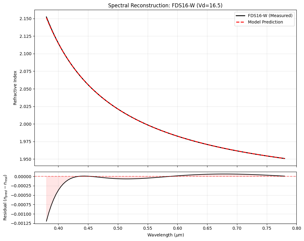
5. Model Validation and Error Analysis
To quantify the predictive fidelity of our derived model, we evaluate the reconstruction error across the full dataset of standard optical glasses.
Methodology: We test the model’s generative capacity by reconstructing the refractive index of each glass in the catalog using only its \(n_d\) and \(V_d\) parameters. This simulates the real-world usage of the data-based model implementation. 1. Input: Extract \(n_d\) and \(V_d\) for every glass. 2. Prediction: Calculate the Buchdahl coefficients (\(v_1, v_2, v_3\)) using the regression weights derived in Section 4. 3. Reconstruction: Generate the full spectral curve \(n(\lambda)\). 4. Validation: Compare against the reference catalog measurements.
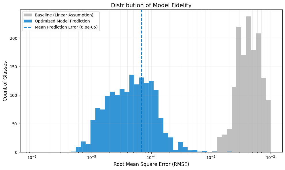
Metric: We track the Root Mean Square Error (RMSE):
We compare this against a Baseline Linear Model, which assumes a simple linear dispersion slope between the F and C lines.
[15]:
# --- 1. Helper Function: The Optimized Model Logic ---
def predict_abbe_index(nd, Vd, wave_grid):
    """
    Reconstructs the refractive index curve using the LASSO-derived coefficients
    from Section 4. This replicates the logic that will go into the new AbbeMaterial class.
    """
    # Buchdahl Constants
    WAVE_D = 0.5875618
    ALPHA = 2.5

    # Feature Engineering (Must match the regression input exactly)
    inv_V = 1.0 / Vd
    inv_V2 = 1.0 / (Vd**2)
    nd_sq = nd**2
    nd_div_V = nd / Vd

    # --- COEFFICIENTS FROM SECTION 4 LASSO ANALYSIS ---

    # Target: v1
    v1 = (0.004160
          + 4.462559 * inv_V
          + 2.326660 * inv_V2
          + 0.002330 * nd
          - 0.003697 * nd_sq
          - 4.697604 * nd_div_V)

    # Target: v2
    v2 = (0.066434
          - 7.636396 * inv_V
          + 12.597434 * inv_V2
          - 0.037014 * nd_sq
          + 5.551013 * nd_div_V)

    # Target: v3
    v3 = (-0.032218
          + 2.230357 * inv_V
          - 103.318994 * inv_V2
          - 0.009654 * nd_sq
          + 1.934983 * nd_div_V)

    # --- Spectral Reconstruction ---
    # Calculate Buchdahl Coordinate omega
    omega = (wave_grid - WAVE_D) / (1 + ALPHA * (wave_grid - WAVE_D))

    # Buchdahl Polynomial: n = nd + sum(vi * omega^i)
    n_pred = nd + v1 * omega + v2 * (omega**2) + v3 * (omega**3)

    return n_pred

# --- 2. Validation Loop ---
rmse_baseline = []
rmse_prediction = []
max_errors = []

print(f"Validating model against {len(df_glass)} catalog glasses...")

for idx, row in df_glass.iterrows():
    # Ground Truth
    n_real = row['curve']

    # Baseline Model (Linear Assumption)
    # Slope defined by F and C lines (Normal Line assumption)
    slope = (row['nd'] - 1) / (row['Vd'] * (WAVE_F - WAVE_C))
    n_baseline = row['nd'] + slope * (WAVE_GRID - WAVE_D)

    # Optimized Model Prediction
    n_pred = predict_abbe_index(row['nd'], row['Vd'], WAVE_GRID)

    # Compute Errors
    error_base = np.sqrt(np.mean((n_baseline - n_real)**2))
    error_pred = np.sqrt(np.mean((n_pred - n_real)**2))

    rmse_baseline.append(error_base)
    rmse_prediction.append(error_pred)

    # Track worst-case spectral error
    max_errors.append(np.max(np.abs(n_pred - n_real)))

# Convert to arrays
rmse_baseline = np.array(rmse_baseline)
rmse_prediction = np.array(rmse_prediction)
max_errors = np.array(max_errors)

print("Validation Loop Complete.")
Validating model against 1678 catalog glasses...
Validation Loop Complete.
[16]:
# Compute Aggregate Statistics
mean_rmse_base = np.mean(rmse_baseline)
mean_rmse_pred = np.mean(rmse_prediction)
improvement_factor = mean_rmse_base / mean_rmse_pred

print("-" * 65)
print(f"GLOBAL VALIDATION STATISTICS (N={len(rmse_prediction)})")
print("-" * 65)
print(f"Baseline (Linear) Mean RMSE:    {mean_rmse_base:.2e}")
print(f"Optimized Model Mean RMSE:      {mean_rmse_pred:.2e}")
print(f"IMPROVEMENT FACTOR:             {improvement_factor:.1f}x reduction in error")
print("-" * 65)
print(f"Avg Max Spectral Error:         {np.mean(max_errors):.2e}")
print("-" * 65)
-----------------------------------------------------------------
GLOBAL VALIDATION STATISTICS (N=1678)
-----------------------------------------------------------------
Baseline (Linear) Mean RMSE:    5.94e-03
Optimized Model Mean RMSE:      6.84e-05
IMPROVEMENT FACTOR:             86.9x reduction in error
-----------------------------------------------------------------
Avg Max Spectral Error:         2.85e-04
-----------------------------------------------------------------
[17]:
plt.figure(figsize=(10, 6))

# Log-spaced bins for wide dynamic range
bins = np.logspace(np.log10(1e-6), np.log10(1e-2), 50)

plt.hist(rmse_baseline, bins=bins, alpha=0.5, color='gray', label='Baseline (Linear Assumption)')
plt.hist(rmse_prediction, bins=bins, alpha=0.8, color='#007acc', label='Optimized Model Prediction')

# Mean Markers
plt.axvline(mean_rmse_pred, color='#007acc', linestyle='--', linewidth=2, label=f'Mean Prediction Error ({mean_rmse_pred:.1e})')

plt.xscale('log')
plt.xlabel('Root Mean Square Error (RMSE)', fontsize=12)
plt.ylabel('Count of Glasses', fontsize=12)
plt.title('Distribution of Model Fidelity', fontsize=14)
plt.legend(loc='upper left')
plt.grid(True, which="both", ls="-", alpha=0.2)

plt.tight_layout()
plt.show()
[18]:
# Select a stress-test glass (Low Abbe number = High Dispersion)
sample_idx = df_glass['Vd'].idxmin()
sample = df_glass.iloc[sample_idx]

# 1. Get Ground Truth
n_real_sample = sample['curve']

# 2. Generate Prediction
n_pred_sample = predict_abbe_index(sample['nd'], sample['Vd'], WAVE_GRID)

# 3. Calculate Residual
residual = n_pred_sample - n_real_sample

# 4. Plot
fig, (ax1, ax2) = plt.subplots(2, 1, figsize=(10, 8), sharex=True, gridspec_kw={'height_ratios': [3, 1]})

# Top: Absolute Index
ax1.plot(WAVE_GRID, n_real_sample, 'k-', linewidth=2, label=f"{sample['name']} (Measured)")
ax1.plot(WAVE_GRID, n_pred_sample, 'r--', linewidth=2, label='Model Prediction')
ax1.set_ylabel('Refractive Index')
ax1.set_title(f"Spectral Reconstruction: {sample['name']} (Vd={sample['Vd']:.1f})")
ax1.legend()
ax1.grid(True, alpha=0.3)

# Bottom: Residual
ax2.plot(WAVE_GRID, residual, 'k-')
ax2.fill_between(WAVE_GRID, residual, 0, color='red', alpha=0.1)

ax2.axhline(0, color='r', linestyle='--', alpha=0.5)

ax2.set_ylabel('Residual ($n_{pred} - n_{real}$)')
ax2.set_xlabel(r'Wavelength ($\mu m$)')
ax2.grid(True, alpha=0.3)

plt.tight_layout()
plt.show()
6. Production Implementation
We now implement the final OptimizedAbbeMaterial class. This class incorporates the specific LASSO-derived coefficients found in the discovery phase.
Key Features: * Hardcoded Physics: The regression weights are baked into the class. * Buchdahl Engine: Uses the robust coordinate transformation \(\omega\) for spectral stability. * Vectorized: Built on the Optiland backend to support efficient array operations during ray tracing.
The code below defines the class and demonstrates its usage by comparing the “Model N-SF11” (generated purely from \(n_d=1.785, V_d=25.7\)) against the actual measured data for N-SF11.
[19]:
import optiland.backend as be
from optiland.materials.base import BaseMaterial
from optiland.materials import Material

class OptimizedAbbeMaterial(BaseMaterial):
    """
    A High-Accuracy Data-Driven Model Glass.

    Predicts the full dispersion curve from only n_d and V_d using a
    statistical prior derived from catalog glass data.

    Attributes:
        index (float): Refractive index at d-line (587.56 nm)
        abbe (float): Abbe number (Vd)
    """

    def __init__(self, n, abbe):
        super().__init__()
        self.index = be.array([n])
        self.abbe = be.array([abbe])
        self._coeffs = self._predict_coefficients()

    def _predict_coefficients(self):
        """
        Calculates Buchdahl coefficients (v1, v2, v3) using the
        equations found via LASSO regression.
        """
        # 1. Feature Engineering
        inv_V = 1.0 / self.abbe
        inv_V2 = inv_V ** 2
        nd = self.index
        nd_sq = nd ** 2
        nd_div_V = nd * inv_V

        # 2. The Discovered Physics Equations

        # Target: v1 (Primary Slope)
        v1 = (0.004160
              + 4.462559 * inv_V
              + 2.326660 * inv_V2
              + 0.002330 * nd
              - 0.003697 * nd_sq
              - 4.697604 * nd_div_V)

        # Target: v2 (Curvature)
        v2 = (0.066434
              - 7.636396 * inv_V
              + 12.597434 * inv_V2
              - 0.037014 * nd_sq
              + 5.551013 * nd_div_V)

        # Target: v3 (Deep Blue Correction)
        v3 = (-0.032218
              + 2.230357 * inv_V
              - 103.318994 * inv_V2
              - 0.009654 * nd_sq
              + 1.934983 * nd_div_V)

        return v1, v2, v3

    def _calculate_n(self, wavelength, **kwargs):
        wavelength = be.array(wavelength)

        # Buchdahl Coordinate Transformation (d-line centered)
        # w = (lam - 0.58756) / (1 + 2.5 * (lam - 0.58756))
        lam_norm = wavelength - 0.5875618
        w = lam_norm / (1.0 + 2.5 * lam_norm)

        v1, v2, v3 = self._coeffs

        # n(w) = nd + v1*w + v2*w^2 + v3*w^3
        return self.index + v1 * w + v2 * (w**2) + v3 * (w**3)

    def _calculate_k(self, wavelength, **kwargs):
        return be.zeros_like(wavelength)

    def to_dict(self):
        material_dict = super().to_dict()
        material_dict.update({"index": float(self.index), "abbe": float(self.abbe)})
        return material_dict
[ ]:
# We verify the model against a difficult high-index flint (N-SF11)
glass_name = "N-SF11"
real_glass = Material(glass_name)

# 1. Create the Model Glass using ONLY nd and Vd
nd_val = real_glass.n(0.5875618).item()
Vd_val = real_glass.abbe().item()
model_glass = OptimizedAbbeMaterial(nd_val, Vd_val)

print(f"Demonstration: Modeling {glass_name}")
print(f"Inputs: nd={nd_val:.4f}, Vd={Vd_val:.2f}")

# 2. Calculate Curves
wave_grid = np.linspace(0.38, 0.78, 500)
n_real = real_glass.n(wave_grid)
n_model = model_glass.n(wave_grid)
residual = n_model - n_real

# 3. Visualize
fig, (ax1, ax2) = plt.subplots(2, 1, figsize=(10, 8), sharex=True, gridspec_kw={'height_ratios': [3, 1]})

# Top: Absolute Index
ax1.plot(wave_grid, n_real, 'k-', linewidth=2, label=f'{glass_name} (Measured)')
ax1.plot(wave_grid, n_model, 'r--', linewidth=2, label='Optimized Model (Predicted)')
ax1.set_ylabel('Refractive Index')
ax1.set_title(f'Model Reconstruction of {glass_name} (Vd={Vd_val:.1f})')
ax1.legend()
ax1.grid(True, alpha=0.3)

# Bottom: Residual Error
ax2.plot(wave_grid, residual, 'k-')
ax2.fill_between(wave_grid, residual, 0, color='red', alpha=0.1)

ax2.axhline(0, color='r', linestyle='--', alpha=0.5)

ax2.set_ylabel('Residual ($n_{pred} - n_{real}$)')
ax2.set_xlabel(r'Wavelength ($\mu m$)')
ax2.grid(True, alpha=0.3)

plt.tight_layout()
plt.show()
Demonstration: Modeling N-SF11
Inputs: nd=1.7847, Vd=25.68

6. Conclusions
This notebook has successfully derived and validated the AbbeMaterial implementation for Optiland. By applying data science techniques to the physics of optical dispersion, we have moved beyond traditional heuristic models.
Key Results
Sparse Representation: The LassoLarsIC analysis demonstrated that the full spectral behavior of standard glasses can be accurately reconstructed using a sparse subset of Buchdahl terms.
Basis Validity: The PCA decomposition confirms that the refractive index curves of glasses in this study lie on a low-dimensional manifold. This justifies the use of a constrained model (the optimized Buchdahl form) rather than a free-form interpolation.
Justification of Approach
We utilize a data-driven optimization of the Buchdahl Dispersion Model rather than direct polynomial interpolation (e.g., solving for Sellmeier coefficients) for two primary reasons:
Numerical Stability (Convexity): solving for polynomial coefficients (like Sellmeier \(B_i, C_i\)) from limited data points is a non-convex problem. Small changes in inputs (\(n_d, V_d\)) can result in large, chaotic jumps in coefficients, leading to singularities. The Buchdahl coordinate \(\omega\), by contrast, orthogonalizes the spectral space, ensuring that the mapping from (\(n_d, V_d\)) to the dispersion curve remains smooth and continuous.
Parsimony (Occam’s Razor): By using Lasso regression, we strictly enforce sparsity. The model includes only the dispersion terms necessary to describe the variance in the training data, discarding higher-order terms that contribute to overfitting (ringing) at the spectral edges. This ensures the
AbbeMaterialbehaves predictably even when simulating glasses outside the standard catalog range.