Tutorial 7b - Surface Roughness & Scattering

This tutorial demonstrates how surface roughness and scattering can be configured on surfaces in Optiland. We will compare singlets with the following scattering properties assigned:

• No scattering

• Gaussian Scattering

• Lambertian Scattering

The scattering model is defined via the Bidirectional Scattering Distribution Function, or BSDF.

import matplotlib.pyplot as plt
import numpy as np

from optiland import optic, scatter

Preparation

We first define a generic singlet class that accepts a bsdf as an input. In this example, we assign the scattering only to the rear surface.

class SingletConfigurable(optic.Optic):
    def __init__(self, bsdf):
        super().__init__()

        # add surfaces
        self.surfaces.add(index=0, radius=np.inf, thickness=np.inf)
        self.surfaces.add(
            index=1,
            thickness=7,
            radius=50,
            is_stop=True,
            material="N-SF11",
        )
        self.surfaces.add(index=2, thickness=50, bsdf=bsdf)  # <-- add bsdf here
        self.surfaces.add(index=3)

        # add aperture
        self.set_aperture(aperture_type="EPD", value=25.4)

        # add field
        self.fields.set_type(field_type="angle")
        self.fields.add(y=0)
        self.fields.add(y=10)
        self.fields.add(y=14)

        # add wavelength
        self.wavelengths.add(value=0.48613270)
        self.wavelengths.add(value=0.58756180, is_primary=True)
        self.wavelengths.add(value=0.65627250)

        self.image_solve()  # solve for image plane

Let’s also define a helper function to plot a 2D distribution of rays intersection points.

def plot_ray_distribution(rays, bins=128):
    x = rays.x
    y = rays.y
    i = rays.i

    plt.hist2d(x, y, weights=i, bins=bins, cmap="viridis")
    plt.colorbar()
    plt.xlabel("X (mm)")
    plt.ylabel("Y (mm)")
    plt.title("2D Ray Distribution on Image Plane")
    plt.show()

1. Singlet #1 - No Surface Scattering

The first singlet we analyze will have no scattering applied. Let’s first define the lens and draw it.

singlet_no_scatter = SingletConfigurable(bsdf=None)

singlet_no_scatter.draw()

Let’s trace 1 million random rays through the lens at the on-axis field point and look at the distribution.

rays = singlet_no_scatter.trace(
    Hx=0,
    Hy=0,
    wavelength=0.58756180,
    num_rays=1_000_000,
    distribution="random",
)

plot_ray_distribution(rays, bins=128)

As we can see, the energy is largely located at the origin on the image plane. Let’s see how this is implacted when scattering is introduced.

2. Singlet #2 - Gaussian Scattering

Gaussian scattering is defined by a 2D Gaussian distribution with a user-defined sigma (std. dev.) value. The larger the value of sigma, the closer the scattering model comes to Lambertian. We define a GaussianBSDF model with a sigma value of 0.01 and generate a new singlet:

bsdf = scatter.GaussianBSDF(sigma=0.01)
singlet_gaussian = SingletConfigurable(bsdf=bsdf)

Again, we trace 1 million rays and view the distribution at the image plane:

rays = singlet_gaussian.trace(
    Hx=0,
    Hy=0,
    wavelength=0.58756180,
    num_rays=1_000_000,
    distribution="random",
)

plot_ray_distribution(rays)

The image size has blurred significantly in comparison to the no-scattering case. Note that the plot axis spans a larger range here as well.

3. Singlet #3 - Lambertian Scattering

Lambertian scattering implies that the surface scatters incident light uniformly in all directions. Diffuse surfaces can be considered approximately Lambertian. To model a Lambertian scatterer in Optiland, we simply define the LambertianBSDF model and pass it to our singlet:

bsdf = scatter.LambertianBSDF()
singlet_lambertian = SingletConfigurable(bsdf=bsdf)

rays = singlet_lambertian.trace(
    Hx=0,
    Hy=0,
    wavelength=0.58756180,
    num_rays=1_000_000,
    distribution="random",
)

plot_ray_distribution(rays, bins=np.linspace(-100, 100, 128))

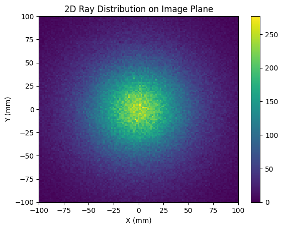
In this case, we are plotting the image plane over a significantly larger area, from -100 mm to 100 mm. Clearly, the Lambertian scatter model has dramatically increased the spot size at the image plane.

4. Conclusions:

• We introduced two BSDF scatter models: Gaussian and Lambertian.

• Scatter models can be used to model and understand the impact of manufacturing defects, such as surface roughness on optical surfaces.