Tutorial 3a - Common aberration analyses
This tutorial demonstrates the various aberration plots and analyses that can be performed in Optiland. Namely, we cover:
Spot diagrams
Ray fans
Y-Ybar plots
Distortion / Grid distortion plots
Field curvature plots
[1]:
from optiland import analysis
from optiland.samples.objectives import CookeTriplet
[2]:
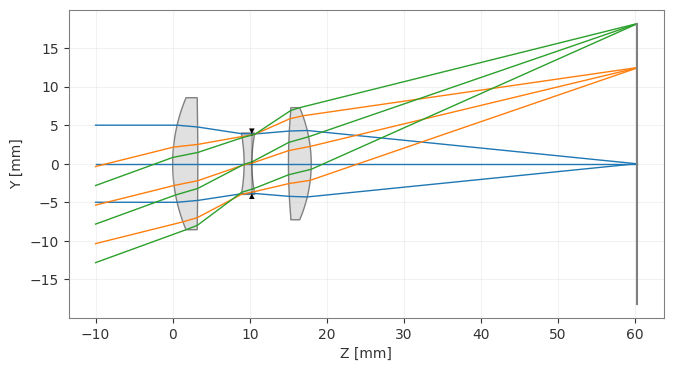
lens = CookeTriplet()
lens.draw()
[2]:
(<Figure size 1000x400 with 1 Axes>, <Axes: xlabel='Z [mm]', ylabel='Y [mm]'>)
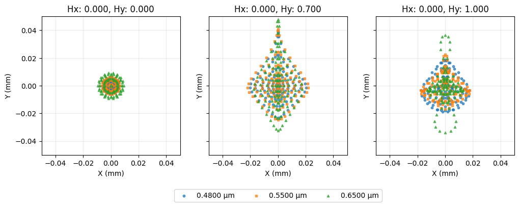
Spot Diagram
[3]:
spot = analysis.SpotDiagram(lens)
spot.view()
[3]:
(<Figure size 1200x400 with 3 Axes>,
 [<Axes: title={'center': 'Hx: 0.000, Hy: 0.000'}, xlabel='X (mm)', ylabel='Y (mm)'>,
  <Axes: title={'center': 'Hx: 0.000, Hy: 0.700'}, xlabel='X (mm)', ylabel='Y (mm)'>,
  <Axes: title={'center': 'Hx: 0.000, Hy: 1.000'}, xlabel='X (mm)', ylabel='Y (mm)'>])
[4]:
fields = lens.fields.get_field_coords()
wavelengths = lens.wavelengths.get_wavelengths()
[5]:
print("Geometric Spot Radius:")

geo_spot_radius = spot.geometric_spot_radius()
for i, field in enumerate(fields):
    for j, wavelength in enumerate(wavelengths):
        print(
            f"\tField {field}, Wavelength {wavelength:.3f} µm, "
            f"Radius: {geo_spot_radius[i][j]:.5f} mm",
        )
Geometric Spot Radius:
        Field (0.0, 0.0), Wavelength 0.480 µm, Radius: 0.00597 mm
        Field (0.0, 0.0), Wavelength 0.550 µm, Radius: 0.00629 mm
        Field (0.0, 0.0), Wavelength 0.650 µm, Radius: 0.00932 mm
        Field (0.0, 0.7), Wavelength 0.480 µm, Radius: 0.03928 mm
        Field (0.0, 0.7), Wavelength 0.550 µm, Radius: 0.04075 mm
        Field (0.0, 0.7), Wavelength 0.650 µm, Radius: 0.04772 mm
        Field (0.0, 1.0), Wavelength 0.480 µm, Radius: 0.01891 mm
        Field (0.0, 1.0), Wavelength 0.550 µm, Radius: 0.02250 mm
        Field (0.0, 1.0), Wavelength 0.650 µm, Radius: 0.03655 mm
[6]:
print("RMS Spot Radius:")

rms_spot_radius = spot.rms_spot_radius()
for i, field in enumerate(fields):
    for j, wavelength in enumerate(wavelengths):
        print(
            f"\tField {field}, Wavelength {wavelength:.3f} µm, "
            f"Radius: {rms_spot_radius[i][j]:.5f} mm",
        )
RMS Spot Radius:
        Field (0.0, 0.0), Wavelength 0.480 µm, Radius: 0.00379 mm
        Field (0.0, 0.0), Wavelength 0.550 µm, Radius: 0.00429 mm
        Field (0.0, 0.0), Wavelength 0.650 µm, Radius: 0.00620 mm
        Field (0.0, 0.7), Wavelength 0.480 µm, Radius: 0.01582 mm
        Field (0.0, 0.7), Wavelength 0.550 µm, Radius: 0.01692 mm
        Field (0.0, 0.7), Wavelength 0.650 µm, Radius: 0.01922 mm
        Field (0.0, 1.0), Wavelength 0.480 µm, Radius: 0.01324 mm
        Field (0.0, 1.0), Wavelength 0.550 µm, Radius: 0.01212 mm
        Field (0.0, 1.0), Wavelength 0.650 µm, Radius: 0.01365 mm
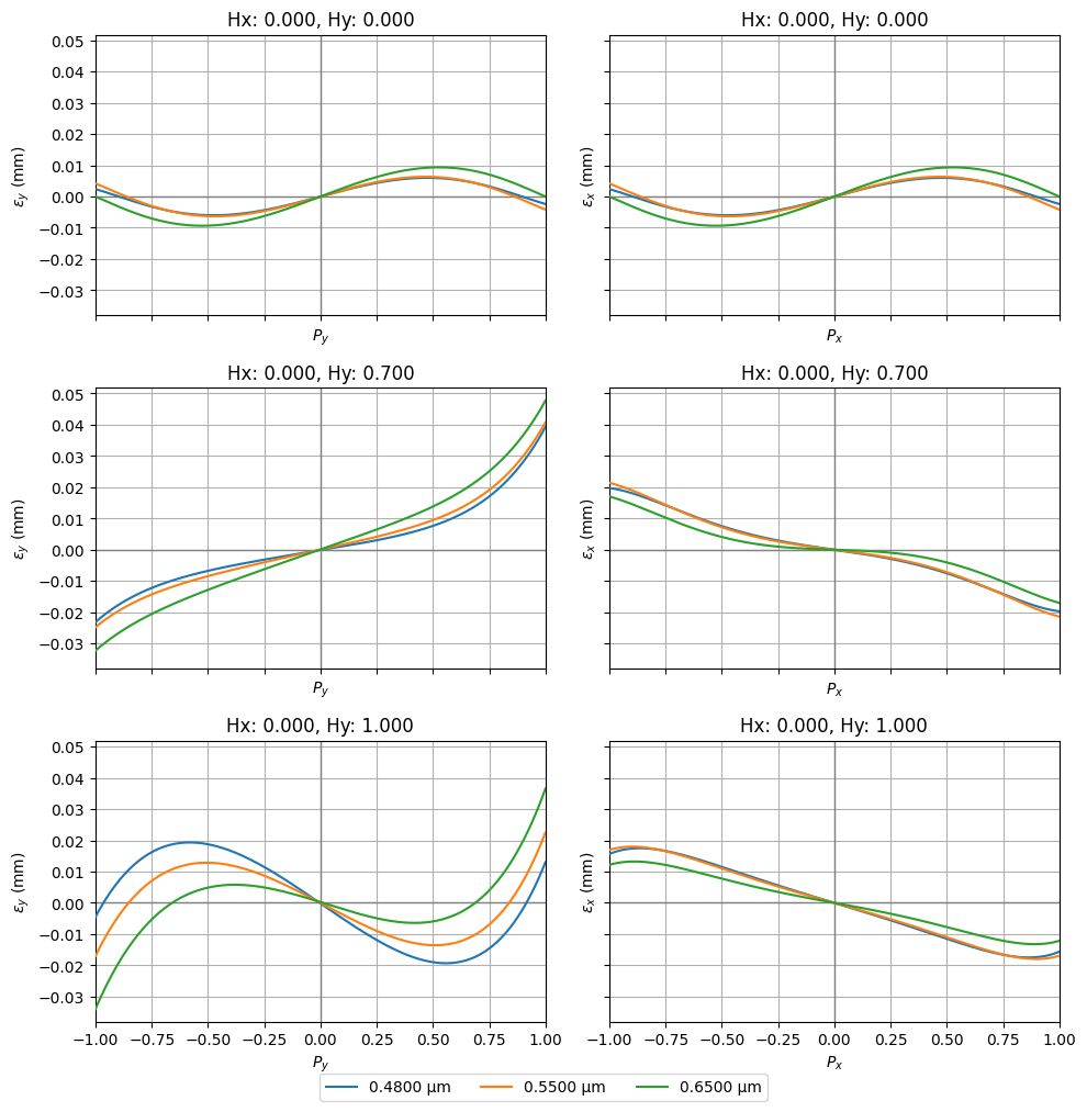
Ray fans
[7]:
fan = analysis.RayFan(lens)
fan.view()
[7]:
(<Figure size 1000x999 with 6 Axes>,
 [<Axes: title={'center': 'Hx: 0.000, Hy: 0.000'}, xlabel='$P_y$', ylabel='$\\epsilon_y$ (mm)'>,
  <Axes: title={'center': 'Hx: 0.000, Hy: 0.000'}, xlabel='$P_x$', ylabel='$\\epsilon_x$ (mm)'>,
  <Axes: title={'center': 'Hx: 0.000, Hy: 0.700'}, xlabel='$P_y$', ylabel='$\\epsilon_y$ (mm)'>,
  <Axes: title={'center': 'Hx: 0.000, Hy: 0.700'}, xlabel='$P_x$', ylabel='$\\epsilon_x$ (mm)'>,
  <Axes: title={'center': 'Hx: 0.000, Hy: 1.000'}, xlabel='$P_y$', ylabel='$\\epsilon_y$ (mm)'>,
  <Axes: title={'center': 'Hx: 0.000, Hy: 1.000'}, xlabel='$P_x$', ylabel='$\\epsilon_x$ (mm)'>])
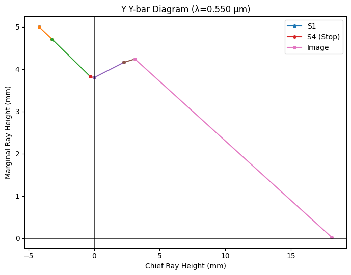
Y-Ybar plot
[8]:
yybar = analysis.YYbar(lens)
yybar.view()
[8]:
(<Figure size 700x550 with 1 Axes>,
 <Axes: title={'center': 'Y Y-bar Diagram (λ=0.550 µm)'}, xlabel='Chief Ray Height (mm)', ylabel='Marginal Ray Height (mm)'>)
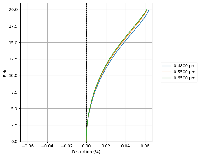
Distortion
[9]:
distortion = analysis.Distortion(lens)
distortion.view()
[9]:
(<Figure size 700x550 with 1 Axes>,
 <Axes: xlabel='Distortion (%)', ylabel='Field'>)
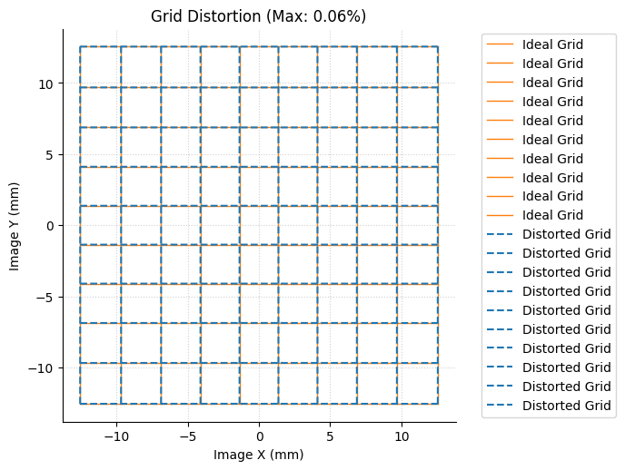
Grid distortion
[10]:
grid = analysis.GridDistortion(lens)
grid.view()
[10]:
(<Figure size 700x700 with 1 Axes>,
 <Axes: title={'center': 'Grid Distortion (Max: 0.06%)'}, xlabel='Image X (mm)', ylabel='Image Y (mm)'>)
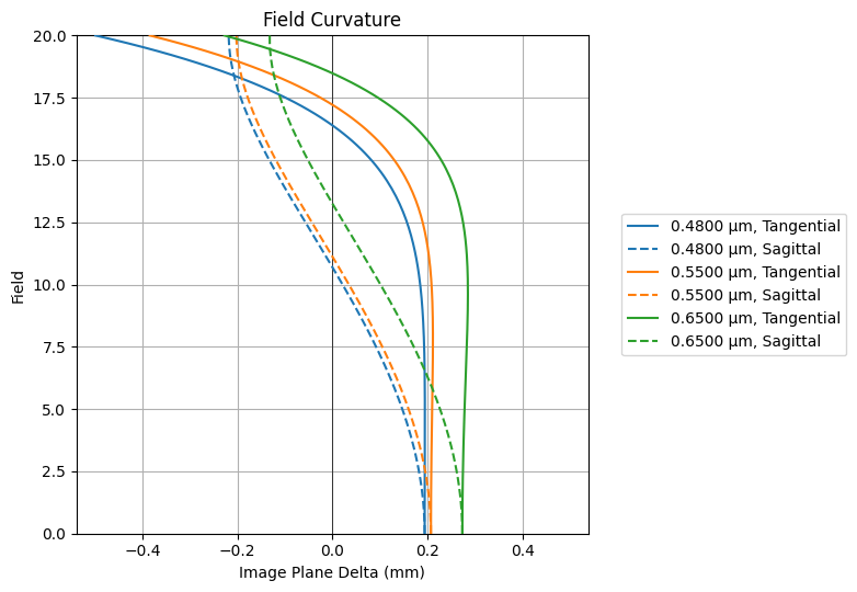
Field Curvature
[11]:
field_curv = analysis.FieldCurvature(lens)
field_curv.view()
[11]:
(<Figure size 800x550 with 1 Axes>,
 <Axes: title={'center': 'Field Curvature'}, xlabel='Image Plane Delta (mm)', ylabel='Field'>)
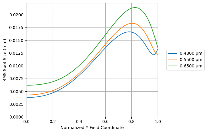
RMS Spot Size vs. Field
[12]:
rms_spot_vs_field = analysis.RmsSpotSizeVsField(lens)
rms_spot_vs_field.view()
[12]:
(<Figure size 700x450 with 1 Axes>,
 <Axes: xlabel='Normalized Y Field Coordinate', ylabel='RMS Spot Size (mm)'>)
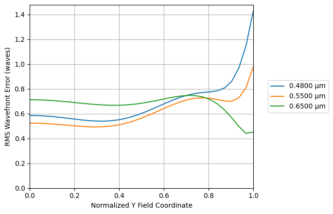
RMS Wavefront Error vs. Field
[13]:
rms_wavefront_error_vs_field = analysis.RmsWavefrontErrorVsField(lens)
rms_wavefront_error_vs_field.view()
[13]:
(<Figure size 700x450 with 1 Axes>,
 <Axes: xlabel='Normalized Y Field Coordinate', ylabel='RMS Wavefront Error (waves)'>)
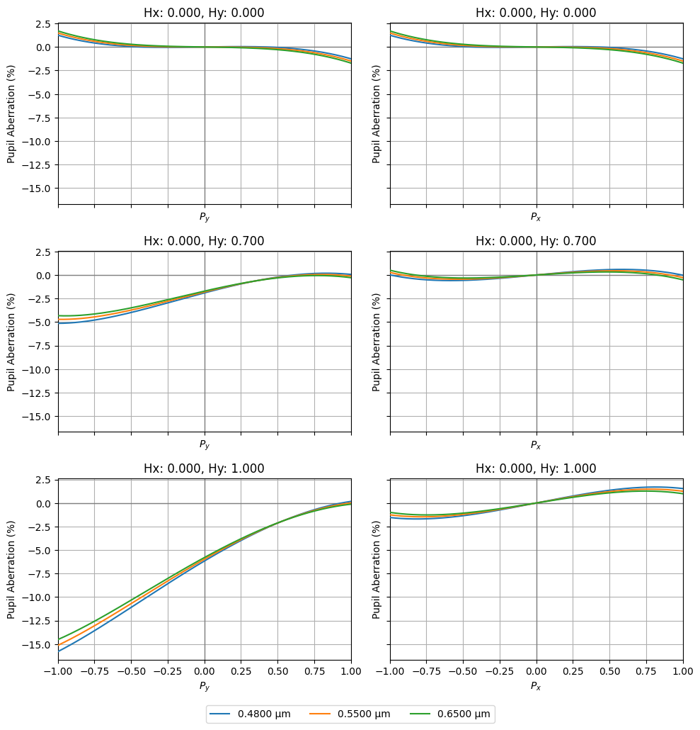
Pupil Aberration
The pupil abberration is defined as the difference between the paraxial and real ray intersection point at the stop surface of the optic. This is specified as a percentage of the on-axis paraxial stop radius at the primary wavelength.
[14]:
pupil_ab = analysis.PupilAberration(lens)
pupil_ab.view()
[14]:
(<Figure size 1000x999 with 6 Axes>,
 array([[<Axes: title={'center': 'Hx: 0.000, Hy: 0.000'}, xlabel='$P_y$', ylabel='Pupil Aberration (%)'>,
         <Axes: title={'center': 'Hx: 0.000, Hy: 0.000'}, xlabel='$P_x$', ylabel='Pupil Aberration (%)'>],
        [<Axes: title={'center': 'Hx: 0.000, Hy: 0.700'}, xlabel='$P_y$', ylabel='Pupil Aberration (%)'>,
         <Axes: title={'center': 'Hx: 0.000, Hy: 0.700'}, xlabel='$P_x$', ylabel='Pupil Aberration (%)'>],
        [<Axes: title={'center': 'Hx: 0.000, Hy: 1.000'}, xlabel='$P_y$', ylabel='Pupil Aberration (%)'>,
         <Axes: title={'center': 'Hx: 0.000, Hy: 1.000'}, xlabel='$P_x$', ylabel='Pupil Aberration (%)'>]],
       dtype=object))