Tutorial 11a: Extended Source Modeling

This tutorial demonstrates how to use the ExtendedSourceOptic feature to model extended sources in Optiland. We will simulate the irradiance profile of a beam shaping singlet with a collimated Gaussian extended source.

Key concepts covered: 1. Defining a custom optical system. 2. Setting up an extended source using SMFSource (Single-Mode Fiber Source). 3. Integrating the source with the optical system using ExtendedSourceOptic. 4. Visualizing the system with source rays. 5. Analysing the output irradiance.

import optiland.backend as be
from optiland.optic import Optic, ExtendedSourceOptic
from optiland.sources import SMFSource
from optiland.analysis import IncoherentIrradiance
from optiland.physical_apertures import RectangularAperture

1. Define the Optical System

First, we define the Beam Shaping Singlet system. This system is designed to transform a Gaussian beam into a flat-top profile.

gaussian_beam_waist = 5.0  # in mm
wavelength_um = 0.55  # in µm

# Forbes QBFS surface parameters
forbes_terms = {
    0: 0.5414,
    1: 0.6689,
    2: 0.3409,
    3: -0.0537,
    4: -0.3960,
    5: -0.2991,
    6: 0.3921,
}
forbes_norm_radius = 30.3636
top_hat_radius = 25.0

# Create the Optic
lens = Optic()
lens.set_aperture(
    aperture_type="EPD", value=gaussian_beam_waist * 6
)
lens.wavelengths.add(value=wavelength_um, is_primary=True)
lens.fields.set_type(field_type="angle")
lens.fields.add(y=0.0)

# Add surfaces
lens.surfaces.add(index=0, thickness=be.inf)
lens.surfaces.add(
    index=1,
    thickness=20.0,
    is_stop=True,
    aperture=RectangularAperture(
        x_min=-15,
        x_max=15,
        y_min=-15,
        y_max=15,
    ),
)
lens.surfaces.add(
    index=2,
    surface_type="forbes_qbfs",
    radius=5.7410,
    conic=-2.3165,
    thickness=15.0,
    material="N-BK7",
    radial_terms=forbes_terms,
    norm_radius=forbes_norm_radius,
    aperture=30.0,
)
lens.surfaces.add(
    index=3,
    surface_type="standard",
    radius=be.inf,
    thickness=70.0,
    material="air"
)
lens.surfaces.add(
    index=4,
    aperture=RectangularAperture(
        x_min=-top_hat_radius * 1.1,
        x_max=top_hat_radius * 1.1,
        y_min=-top_hat_radius * 1.1,
        y_max=top_hat_radius * 1.1,
    ),
)

Note on Normalization Radius (``norm_radius``):

In optiland, when you explicitly provide normalization parameters (like norm_radius for Forbes/Zernike surfaces, or norm_x/norm_y for Chebyshev surfaces) during geometry initialization, the surface’s normalization_mode is automatically set to 'manual'.

This means the radius is locked to your provided value and will not be automatically scaled during paraxial updates. If you omit the normalization parameters, the normalization_mode defaults to 'auto', and the normalization radius will dynamically scale to \(1.25 \times \text{semi-aperture}\).

2. Setup Extended Source

We use SMFSource to represent a collimated Gaussian source.

Note on Collimation: To approximate a collimated source using SMFSource, we set the divergence angle to an extremely small value (e.g., 1e-10 degrees). The Mode Field Diameter (MFD) determines the spatial extent of the beam. Here we set it to \(2 × \text{waist} = 10\text{ mm} = 10000\text{ µm}\).

# MFD is in microns. 2 * waist (5mm) = 10mm = 10000um
mfd_microns = gaussian_beam_waist * 2 * 1000

# Create the source
source = SMFSource(
    mfd_um=mfd_microns,
    wavelength_um=wavelength_um,
    divergence_deg_1e2=1e-10,  # Virtually zero divergence for collimation
    total_power=1.0,
    position=(0, 0, 0)
)

# Wrap the optic with the source
ext_optic = ExtendedSourceOptic(lens, source)

print(source)

SMFSource(mfd=10000.0µm, divergence=1e-10°, wavelength=0.55µm, power=1.0W, mode=extended, position=(0.0, 0.0, 0.0))

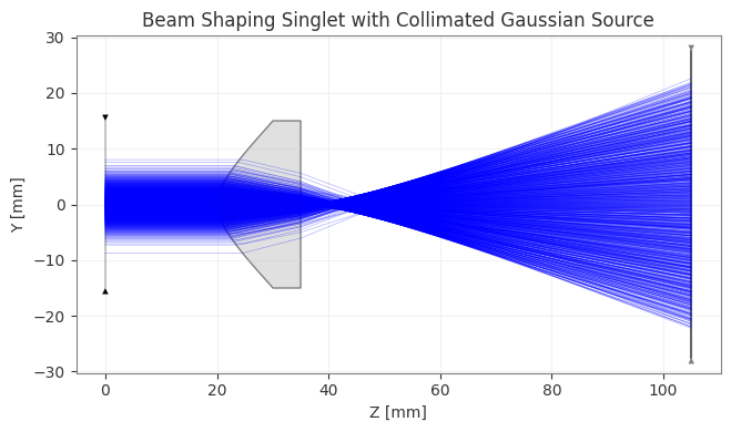
3. Visualization

We can now draw the optical system with the source rays traced through it. The draw method of ExtendedSourceOptic handles this automatically.

fig, ax = ext_optic.draw(num_rays=1000, title="Beam Shaping Singlet with Collimated Gaussian Source")
fig.show()

C:\Users\kdani\AppData\Local\Temp\ipykernel_1988\284778195.py:2: UserWarning: FigureCanvasAgg is non-interactive, and thus cannot be shown
  fig.show()

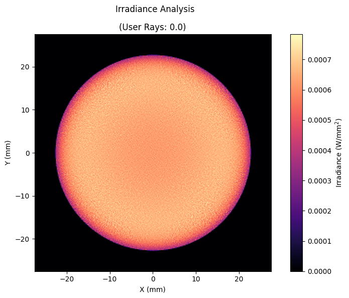
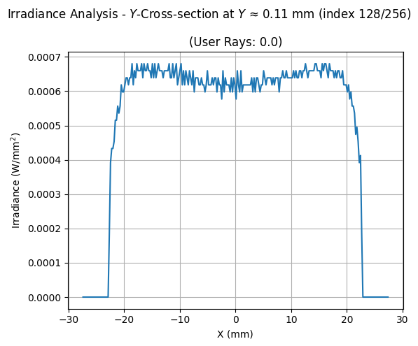
4. Irradiance Analysis

Finally, we calculate and visualize the irradiance at the image plane. We trace a larger number of rays for better resolution and use IncoherentIrradiance.

# Compute and plot irradiance
analysis = IncoherentIrradiance(lens, source=source, num_rays=1_000_000, detector_surface=-1, res=(256, 256))
analysis.view(figsize=(8, 6), cmap="magma", normalize=False)
analysis.view(cross_section=("cross-y", 128), normalize=False)

(<Figure size 600x500 with 1 Axes>,
 array([[<Axes: title={'center': '(User Rays: 0.0)'}, xlabel='X (mm)', ylabel='Irradiance (W/mm$^2$)'>]],
       dtype=object))