Tutorial 5c: Thin Film Optimization and Needle Synthesis

Consolidating active optimization of thin film stacks and automated needle synthesis.

from optiland.thin_film.optimization import ThinFilmOptimizer
import optiland.backend as be
from optiland.thin_film import ThinFilmStack, SpectralAnalyzer
from optiland.materials import Material, IdealMaterial

SiO2 = Material("SiO2", reference="Gao")
TiO2 = Material("TiO2", reference="Zhukovsky")
BK7 = Material("N-BK7", reference="SCHOTT")
air = IdealMaterial(n=1.0)

dichroic_stack = ThinFilmStack(
    incident_material=air,
    substrate_material=BK7,
    reference_wl_um=0.6,
    reference_AOI_deg=45.0,
)
for i in range(10):  # 10 pairs = 20 layers
    dichroic_stack.add_layer_qwot(material=TiO2, qwot_thickness=1.0, name=f"$TiO_2$")
    dichroic_stack.add_layer_qwot(material=SiO2, qwot_thickness=1.0, name=f"$SiO_2$")

optimizer = ThinFilmOptimizer(dichroic_stack)

# Add all thicknesses as optimization variables
for i in range(len(dichroic_stack.layers)):
    optimizer.add_variable(
        layer_index=i,
        min_nm=30,
        max_nm=300
    )

# we want to maximize the polarization contrast (Rs-Rp) at 600 nm and 45° AOI, so we
# minimize the negative contrast, averaged over a wavelength range to make it more
# robust to fabrication variations. The contrast is normalized to be between 0 and 1,
# where 1 corresponds to Rs=1 and Rp=0
wl_nm = be.linspace(595, 605, 11)

# Register and add a custom operand through add_operand
def polarization_contrast(stack: ThinFilmStack, wavelength_nm: be.ndarray, aoi_deg:float):
    """Calculate the polarization contrast (Rs-Rp) averaged over a wavelength range.
    The contrast is normalized to be between 0 and 1, where 1 corresponds to Rs=1 and Rp=0."""
    rs = stack.reflectance_nm_deg(wavelength_nm, aoi_deg, "s")
    rp = stack.reflectance_nm_deg(wavelength_nm, aoi_deg, "p")
    return (1 + be.mean(rs - rp))/2

ThinFilmOptimizer.register_operand(
    "polarization_contrast", polarization_contrast, overwrite=True
)

optimizer.add_operand(
    property="polarization_contrast",
    min_val=0.99,
    input_data={"wavelength_nm": wl_nm, "aoi_deg": 45.0},
    label="Rs-Rp @ 595-605nm, 45deg",
)

# Display optimization information
optimizer.info()
contrast_initial=optimizer.rss()
print(f"Initial RSS: {contrast_initial:.6e}")

ThinFilm Optimizer Information
==================================================
+--------------+---------+
| Property     |   Count |
+==============+=========+
| Stack layers |      20 |
+--------------+---------+
| Variables    |      20 |
+--------------+---------+
| Targets      |       1 |
+--------------+---------+

Variables:
+------+---------+------------------+------------+------------+
|   ID |   Layer |   Thickness (nm) |   Min (nm) |   Max (nm) |
+======+=========+==================+============+============+
|    0 |       0 |             88.2 |         30 |        300 |
+------+---------+------------------+------------+------------+
|    1 |       1 |            143.6 |         30 |        300 |
+------+---------+------------------+------------+------------+
|    2 |       2 |             88.2 |         30 |        300 |
+------+---------+------------------+------------+------------+
|    3 |       3 |            143.6 |         30 |        300 |
+------+---------+------------------+------------+------------+
|    4 |       4 |             88.2 |         30 |        300 |
+------+---------+------------------+------------+------------+
|    5 |       5 |            143.6 |         30 |        300 |
+------+---------+------------------+------------+------------+
|    6 |       6 |             88.2 |         30 |        300 |
+------+---------+------------------+------------+------------+
|    7 |       7 |            143.6 |         30 |        300 |
+------+---------+------------------+------------+------------+
|    8 |       8 |             88.2 |         30 |        300 |
+------+---------+------------------+------------+------------+
|    9 |       9 |            143.6 |         30 |        300 |
+------+---------+------------------+------------+------------+
|   10 |      10 |             88.2 |         30 |        300 |
+------+---------+------------------+------------+------------+
|   11 |      11 |            143.6 |         30 |        300 |
+------+---------+------------------+------------+------------+
|   12 |      12 |             88.2 |         30 |        300 |
+------+---------+------------------+------------+------------+
|   13 |      13 |            143.6 |         30 |        300 |
+------+---------+------------------+------------+------------+
|   14 |      14 |             88.2 |         30 |        300 |
+------+---------+------------------+------------+------------+
|   15 |      15 |            143.6 |         30 |        300 |
+------+---------+------------------+------------+------------+
|   16 |      16 |             88.2 |         30 |        300 |
+------+---------+------------------+------------+------------+
|   17 |      17 |            143.6 |         30 |        300 |
+------+---------+------------------+------------+------------+
|   18 |      18 |             88.2 |         30 |        300 |
+------+---------+------------------+------------+------------+
|   19 |      19 |            143.6 |         30 |        300 |
+------+---------+------------------+------------+------------+

Targets:
+------+--------------------------+--------+---------+--------------+-------+----------+-------+
|   ID | Prop                     | Type   | Value   | Wavelength   | AOI   |   Weight | Pol   |
+======+==========================+========+=========+==============+=======+==========+=======+
|    0 | Rs-Rp @ 595-605nm, 45deg | custom |         | -            | -     |        1 | -     |
+------+--------------------------+--------+---------+--------------+-------+----------+-------+

Initial RSS: 3.058333e-01

# Launch optimization
result = optimizer.optimize(
    method="L-BFGS-B",
    max_iterations=1000,
)

print(f"Merit: {result['initial_merit']:.15f} -> {result['final_merit']:.15f} in {result['iterations']} iterations")
print(f"Improvement: {result['improvement']:.15f}")

Merit: 0.093534002618582 -> 0.000329856133348 in 46 iterations
Improvement: 0.093204146485235

from optiland.thin_film.optimization import ThinFilmReport

report = ThinFilmReport(optimizer, result)
report.summary_table()

	Variable	Initial	Final	Change	Unit
0	Layer 0 thickness	88.2	71.4	-16.8 (-19.1%)	nm
1	Layer 1 thickness	143.6	145.8	+2.2 (+1.5%)	nm
2	Layer 2 thickness	88.2	78.3	-9.9 (-11.2%)	nm
3	Layer 3 thickness	143.6	153.6	+10.0 (+7.0%)	nm
4	Layer 4 thickness	88.2	199.6	+111.4 (+126.3%)	nm
5	Layer 5 thickness	143.6	146.2	+2.6 (+1.8%)	nm
6	Layer 6 thickness	88.2	74.2	-14.1 (-16.0%)	nm
7	Layer 7 thickness	143.6	135.6	-8.0 (-5.6%)	nm
8	Layer 8 thickness	88.2	72.0	-16.2 (-18.4%)	nm
9	Layer 9 thickness	143.6	132.5	-11.1 (-7.7%)	nm
10	Layer 10 thickness	88.2	70.8	-17.4 (-19.8%)	nm
11	Layer 11 thickness	143.6	132.5	-11.1 (-7.7%)	nm
12	Layer 12 thickness	88.2	67.3	-20.9 (-23.7%)	nm
13	Layer 13 thickness	143.6	161.4	+17.8 (+12.4%)	nm
14	Layer 14 thickness	88.2	196.0	+107.7 (+122.1%)	nm
15	Layer 15 thickness	143.6	161.7	+18.1 (+12.6%)	nm
16	Layer 16 thickness	88.2	77.6	-10.7 (-12.1%)	nm
17	Layer 17 thickness	143.6	137.2	-6.4 (-4.5%)	nm
18	Layer 18 thickness	88.2	71.3	-16.9 (-19.1%)	nm
19	Layer 19 thickness	143.6	140.0	-3.6 (-2.5%)	nm

import matplotlib.pyplot as plt

analyzer = SpectralAnalyzer(dichroic_stack)
fig, axes = plt.subplots(1, 3, figsize=(12, 4))

wl_range = be.linspace(500, 700, 201)  # Around 600 nm

# Calculate before optimization (reset and recalculate)
optimizer.reset()
Rs_before = dichroic_stack.reflectance_nm_deg(wl_range, 45, 's')
Rp_before = dichroic_stack.reflectance_nm_deg(wl_range, 45, 'p')

# Restore optimized state
for i, var_info in enumerate(optimizer.variables):
    final_thickness = result['thickness_changes'][i]['final_nm'] / 1000  # nm → μm
    dichroic_stack.layers[i].update_thickness(final_thickness)

Rs_after = dichroic_stack.reflectance_nm_deg(wl_range, 45, 's')
Rp_after = dichroic_stack.reflectance_nm_deg(wl_range, 45, 'p')

axes[0].plot(wl_range, Rs_before, 'b:', label='$R_s$ before', alpha=0.7)
axes[0].plot(wl_range, Rp_before, 'g:', label='$P_p$ before', alpha=0.7)
axes[0].plot(wl_range, Rs_after, 'b-', label='$R_s$ after', linewidth=2)
axes[0].plot(wl_range, Rp_after, 'g-', label='$P_p$ after', linewidth=2)
axes[0].set_xlabel('$\lambda$ (nm)')
axes[0].set_ylabel('Reflectance')
axes[0].set_title('Spectral Performance (AOI=45°)')
axes[0].legend()
axes[0].grid(True, alpha=0.3)
axes[0].fill_betweenx([0, 1], 595, 605, color='gray', alpha=0.2, label='Optimization Range')

# 2. Polarization contrast (Rs - Rp)
contrast_before = Rs_before - Rp_before
contrast_after = Rs_after - Rp_after

axes[1].plot(wl_range, contrast_before, 'g--', label='Before', alpha=0.7)
axes[1].plot(wl_range, contrast_after, 'g-', label='After', linewidth=2)
axes[1].set_xlabel('$\lambda$ (nm)')
axes[1].set_ylabel('Contrast ($R_s - R_p$)')
axes[1].set_title('Polarization Contrast')
axes[1].legend()
axes[1].grid(True, alpha=0.3)

# 3. Optimized stack structure
dichroic_stack.plot_structure_thickness(axes[2])
axes[2].set_title('Optimized Stack Structure')
fig.tight_layout()

<>:25: SyntaxWarning: invalid escape sequence '\l'
<>:38: SyntaxWarning: invalid escape sequence '\l'
<>:25: SyntaxWarning: invalid escape sequence '\l'
<>:38: SyntaxWarning: invalid escape sequence '\l'
C:\Users\kdani\AppData\Local\Temp\ipykernel_3984\3268724171.py:25: SyntaxWarning: invalid escape sequence '\l'
  axes[0].set_xlabel('$\lambda$ (nm)')
C:\Users\kdani\AppData\Local\Temp\ipykernel_3984\3268724171.py:38: SyntaxWarning: invalid escape sequence '\l'
  axes[1].set_xlabel('$\lambda$ (nm)')

---

Part 2: Needle Synthesis

import numpy as np
import matplotlib.pyplot as plt
from optiland.materials import Material, IdealMaterial
from optiland.thin_film import ThinFilmStack, SpectralAnalyzer
from optiland.thin_film.optimization import NeedleSynthesis
from optiland.thin_film.optimization.operand.thin_film import ThinFilmOperand

Part 2.1: Broadband AR Coating (R < 1%)

1. Define materials and starting design

We use real dispersive materials from the optiland catalog:

Material	Role	n @ 550 nm	Reference
N-BK7	Substrate	1.519	Schott
SiO2	Low-index layer	1.460	Malitson
TiO2	High-index layer	2.648	Devore
MgF2	Very low-index layer	1.379	Dodge
Al2O3	Mid-index layer	1.770	Malitson

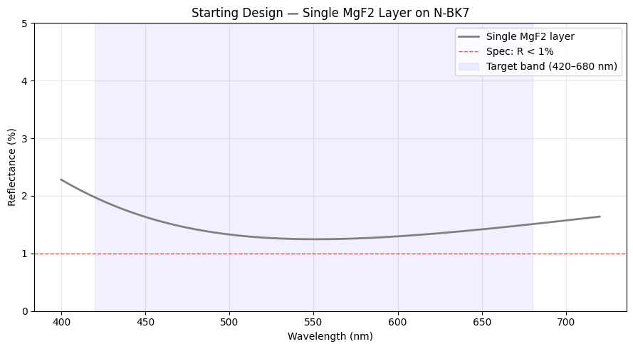
We start from a single MgF2 quarter-wave layer — the simplest possible AR coating. A single low-index layer on N-BK7 gives roughly 1.4% reflectance, which already violates our < 1% spec at the band edges.

# Incident medium
air = IdealMaterial(n=1.0)

# Substrate
nbk7 = Material("N-BK7")

# Candidate coating materials (dispersive)
sio2 = Material("SiO2", reference="Malitson")
tio2 = Material("TiO2", reference="Devore-o")
mgf2 = Material("MgF2", reference="Dodge-o")
al2o3 = Material("Al2O3", reference="Malitson")

# Print refractive indices at 550 nm
for name, mat in [("N-BK7", nbk7), ("SiO2", sio2), ("TiO2", tio2),
                   ("MgF2", mgf2), ("Al2O3", al2o3)]:
    print(f"{name:6s}  n(550nm) = {np.asarray(mat.n(0.55)).item():.4f}")

# Starting design: single MgF2 layer
stack = ThinFilmStack(incident_material=air, substrate_material=nbk7)
stack.add_layer_nm(mgf2, 100.0, name="MgF2")
print("\nStarting design:")
print(stack)

N-BK7   n(550nm) = 1.5185
SiO2    n(550nm) = 1.4599
TiO2    n(550nm) = 2.6479
MgF2    n(550nm) = 1.3785
Al2O3   n(550nm) = 1.7704

Starting design:
ThinFilmStack Summary
---------------------
Incident:  IdealMaterial
Substrate: N-BK7
Layers:
  1. MgF2 (100.0 nm)
---------------------
Total Thickness: 100.0 nm

2. Starting performance

The single MgF2 layer gives ~1.4% average reflectance. The 1% spec line (dashed red) shows the design fails across most of the band.

wl_plot = np.linspace(400, 720, 300)
R_start = np.array([ThinFilmOperand.reflectance(stack, wl) for wl in wl_plot])

fig, ax = plt.subplots(figsize=(9, 5))
ax.plot(wl_plot, R_start * 100, "-", color="gray", linewidth=2, label="Single MgF2 layer")
ax.axhline(1.0, color="red", linestyle="--", linewidth=1, alpha=0.7, label="Spec: R < 1%")
ax.axvspan(420, 680, alpha=0.06, color="blue", label="Target band (420–680 nm)")
ax.set_xlabel("Wavelength (nm)")
ax.set_ylabel("Reflectance (%)")
ax.set_title("Starting Design — Single MgF2 Layer on N-BK7")
ax.set_ylim(0, 5)
ax.legend(loc="upper right")
ax.grid(True, alpha=0.3)
fig.tight_layout();

WARNING: No extinction coefficient data found for Dodge-o.yml. Assuming it is 0.

3. Configure needle synthesis

The algorithm will: 1. Screen trial needle insertions at sampled positions within every layer 2. Try all four candidate materials at each position 3. Insert the needle that reduces the merit function the most 4. Re-optimize all layer thicknesses after each insertion 5. Repeat until no further improvement is found

We target R = 0 at 30 wavelengths across 420–680 nm, driving the optimizer to push reflectance as low as possible everywhere.

ns = NeedleSynthesis(
    stack=stack,
    candidate_materials=[sio2, tio2, mgf2, al2o3],
    needle_thickness_nm=1.0,
    min_thickness_nm=2.0,
    max_iterations=12,
    num_positions_per_layer=8,
    optimizer_max_iter=200,
)

# Dense broadband target: minimize R across 420-680 nm
wavelengths = np.linspace(420, 680, 30).tolist()
ns.add_spectral_target("R", wavelengths, "equal", 0.0)

<optiland.thin_film.optimization.needle.NeedleSynthesis at 0x28e5fb44440>

4. Run needle synthesis

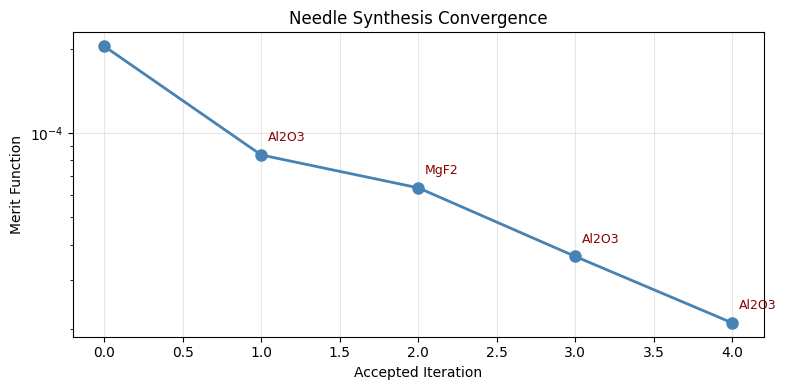
The verbose output shows each iteration: which material was inserted, the needle thickness, and how the merit function evolves.

result = ns.run(verbose=True)

Initial merit after refinement: 2.038637e-04
WARNING: No extinction coefficient data found for Malitson.yml. Assuming it is 0.
WARNING: No extinction coefficient data found for Devore-o.yml. Assuming it is 0.
WARNING: No extinction coefficient data found for Malitson-o.yml. Assuming it is 0.
Iteration 0: TiO2 rejected (merit 1.363746e-02 >= 2.038637e-04)
Iteration 1: inserted Al2O3 (284.2 nm), layers=2, merit = 8.350077e-05
Iteration 2: TiO2 rejected (merit 6.438911e-03 >= 8.350077e-05)
Iteration 3: inserted MgF2 (197.9 nm), layers=4, merit = 6.376946e-05
Iteration 4: TiO2 rejected (merit 1.151474e-02 >= 6.376946e-05)
Iteration 5: TiO2 rejected (merit 1.151447e-02 >= 6.376946e-05)
Iteration 6: TiO2 rejected (merit 2.426760e-03 >= 6.376946e-05)
Iteration 7: inserted Al2O3 (165.4 nm), layers=5, merit = 3.631429e-05
Iteration 8: TiO2 rejected (merit 1.505082e-02 >= 3.631429e-05)
Iteration 9: TiO2 rejected (merit 1.505308e-02 >= 3.631429e-05)
Iteration 10: TiO2 rejected (merit 1.505155e-02 >= 3.631429e-05)
Iteration 11: inserted Al2O3 (168.8 nm), layers=7, merit = 2.104607e-05

5. Results summary

print(f"Success:       {result.success}")
print(f"Iterations:    {result.num_iterations}")
print(f"Layers added:  {result.num_layers_added}")
print(f"Initial merit: {result.initial_merit:.6e}")
print(f"Final merit:   {result.final_merit:.6e}")
print(f"Improvement:   {(1 - result.final_merit / result.initial_merit) * 100:.1f}%")
print(f"\nFinal stack:")
print(result.stack)

# Check against spec: R < 1% everywhere in 420-680 nm
wl_check = np.linspace(420, 680, 100)
R_vals = np.array([ThinFilmOperand.reflectance(result.stack, wl) for wl in wl_check])
print(f"\nAverage R (420-680 nm): {np.mean(R_vals)*100:.3f}%")
print(f"Peak R (420-680 nm):   {np.max(R_vals)*100:.3f}%")
print(f"R < 1% across full band: {np.all(R_vals < 0.01)}")

Success:       True
Iterations:    4
Layers added:  4
Initial merit: 2.038637e-04
Final merit:   2.104607e-05
Improvement:   89.7%

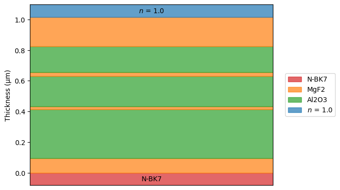
Final stack:
ThinFilmStack Summary
---------------------
Incident:  IdealMaterial
Substrate: N-BK7
Layers:
  1. MgF2 (94.6 nm)
  2. Al2O3 (319.7 nm)
  3. MgF2 (17.7 nm)
  4. Al2O3 (196.1 nm)
  5. MgF2 (26.3 nm)
  6. Al2O3 (170.9 nm)
  7. MgF2 (190.4 nm)
---------------------
Total Thickness: 1015.8 nm

Average R (420-680 nm): 0.388%
Peak R (420-680 nm):   0.990%
R < 1% across full band: True

6. Merit function convergence

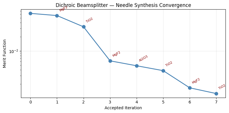
Each accepted needle insertion reduces the merit function. The rollback mechanism ensures rejected insertions (those that worsen performance after re-optimization) are never kept.

merits = [result.initial_merit] + [h.merit_after for h in result.history]
materials_used = [h.material_name for h in result.history]

fig, ax = plt.subplots(figsize=(8, 4))
ax.plot(range(len(merits)), merits, "o-", color="steelblue", linewidth=2, markersize=8)

# Annotate each insertion with material name
for i, (m, name) in enumerate(zip(merits[1:], materials_used), 1):
    ax.annotate(name, (i, m), textcoords="offset points",
                xytext=(5, 10), fontsize=9, color="darkred")

ax.set_xlabel("Accepted Iteration")
ax.set_ylabel("Merit Function")
ax.set_title("Needle Synthesis Convergence")
ax.set_yscale("log")
ax.grid(True, alpha=0.3)
fig.tight_layout();

7. Final stack structure

The algorithm autonomously selected which materials to use and determined the optimal layer thicknesses.

fig, ax = result.stack.plot_structure()

8. Before vs. after comparison

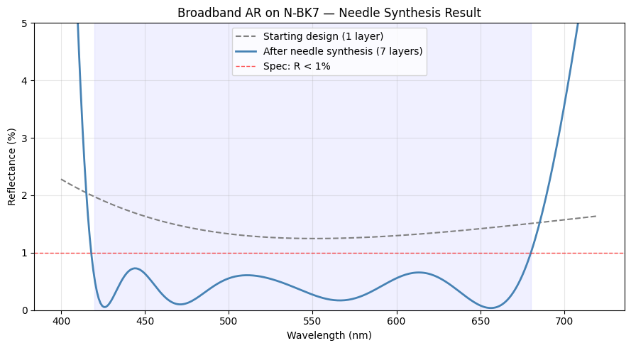
The final design meets the stringent R < 1% spec across the entire 420–680 nm band — something impossible with a single-layer coating on N-BK7.

# Rebuild starting design for comparison
stack_initial = ThinFilmStack(incident_material=air, substrate_material=nbk7)
stack_initial.add_layer_nm(mgf2, 100.0, name="MgF2")

wl_eval = np.linspace(400, 720, 300)
R_initial = np.array([ThinFilmOperand.reflectance(stack_initial, wl) for wl in wl_eval])
R_final = np.array([ThinFilmOperand.reflectance(result.stack, wl) for wl in wl_eval])

fig, ax = plt.subplots(figsize=(9, 5))
ax.plot(wl_eval, R_initial * 100, "--", color="gray",
        linewidth=1.5, label="Starting design (1 layer)")
ax.plot(wl_eval, R_final * 100, "-", color="steelblue",
        linewidth=2, label=f"After needle synthesis ({len(result.stack.layers)} layers)")
ax.axhline(1.0, color="red", linestyle="--", linewidth=1, alpha=0.7, label="Spec: R < 1%")
ax.axvspan(420, 680, alpha=0.06, color="blue")
ax.set_xlabel("Wavelength (nm)")
ax.set_ylabel("Reflectance (%)")
ax.set_title("Broadband AR on N-BK7 — Needle Synthesis Result")
ax.set_ylim(0, 5)
ax.legend()
ax.grid(True, alpha=0.3)
fig.tight_layout();

---

Part 2.2: Dichroic Beamsplitter at 550 nm

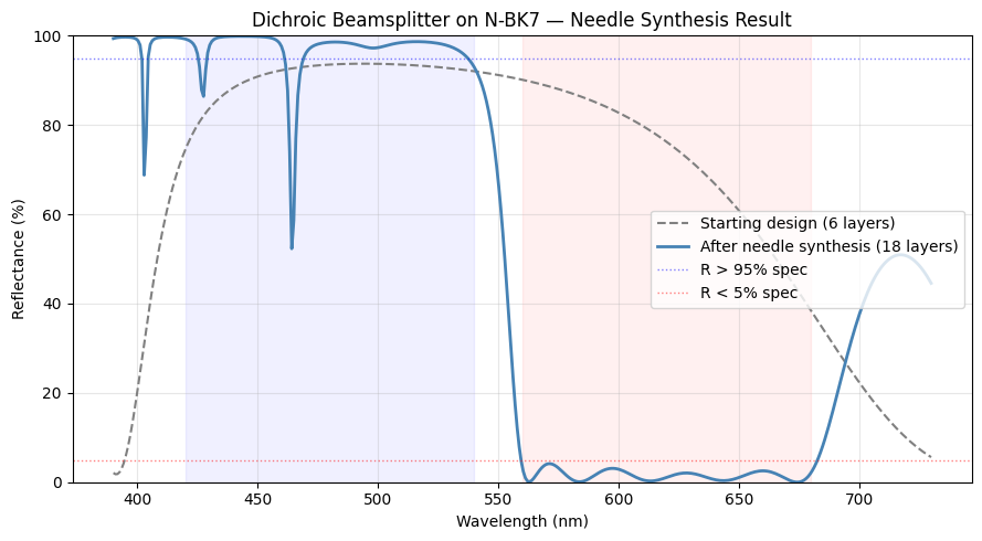
A much harder design problem: a dichroic beamsplitter that reflects blue/green light (420–540 nm) while transmitting orange/red (560–680 nm) with a sharp transition at 550 nm.

Specs: - Reflection band (420–540 nm): R > 95% - Transmission band (560–680 nm): T > 95%

This requires many more layers than a simple AR coating and forces the algorithm to build a complex interference structure from scratch.

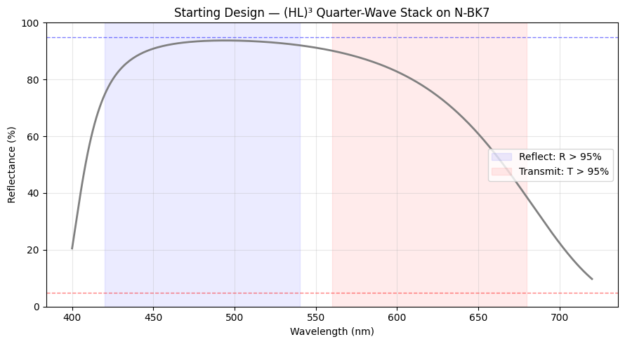
9. Starting design: (HL)^3 quarter-wave stack

We start from a simple 6-layer TiO2/SiO2 quarter-wave stack tuned to 500 nm. This gives some initial reflectance in the blue but is far from meeting spec.

# (HL)^3 quarter-wave stack at 500 nm
# QW optical thickness: n*d = 500/4 = 125 nm
# TiO2 (n~2.65): d = 125/2.65 ~ 47 nm
# SiO2 (n~1.46): d = 125/1.46 ~ 86 nm
stack_d = ThinFilmStack(incident_material=air, substrate_material=nbk7)
for _ in range(3):
    stack_d.add_layer_nm(tio2, 47.0, name="TiO2")
    stack_d.add_layer_nm(sio2, 86.0, name="SiO2")
print(stack_d)

# Plot starting performance
wl_plot = np.linspace(400, 720, 300)
R_start_d = np.array([ThinFilmOperand.reflectance(stack_d, wl) for wl in wl_plot])

fig, ax = plt.subplots(figsize=(9, 5))
ax.plot(wl_plot, R_start_d * 100, "-", color="gray", linewidth=2)
ax.axvspan(420, 540, alpha=0.08, color="blue", label="Reflect: R > 95%")
ax.axvspan(560, 680, alpha=0.08, color="red", label="Transmit: T > 95%")
ax.axhline(95, color="blue", linestyle="--", linewidth=1, alpha=0.5)
ax.axhline(5, color="red", linestyle="--", linewidth=1, alpha=0.5)
ax.set_xlabel("Wavelength (nm)")
ax.set_ylabel("Reflectance (%)")
ax.set_title("Starting Design — (HL)³ Quarter-Wave Stack on N-BK7")
ax.set_ylim(0, 100)
ax.legend(loc="center right")
ax.grid(True, alpha=0.3)
fig.tight_layout();

ThinFilmStack Summary
---------------------
Incident:  IdealMaterial
Substrate: N-BK7
Layers:
  1. TiO2 (47.0 nm)
  2. SiO2 (86.0 nm)
  3. TiO2 (47.0 nm)
  4. SiO2 (86.0 nm)
  5. TiO2 (47.0 nm)
  6. SiO2 (86.0 nm)
---------------------
Total Thickness: 399.0 nm

10. Run needle synthesis for the dichroic

ns_d = NeedleSynthesis(
    stack=stack_d,
    candidate_materials=[sio2, tio2, mgf2, al2o3],
    needle_thickness_nm=1.0,
    min_thickness_nm=2.0,
    max_iterations=8,
    num_positions_per_layer=3,
    optimizer_max_iter=80,
)

# Reflection band: R → 1 for 420-540 nm
wl_reflect = np.linspace(420, 540, 10).tolist()
ns_d.add_spectral_target("R", wl_reflect, "equal", 1.0)

# Transmission band: R → 0 for 560-680 nm
wl_transmit = np.linspace(560, 680, 10).tolist()
ns_d.add_spectral_target("R", wl_transmit, "equal", 0.0)

result_d = ns_d.run(verbose=True)

Initial merit after refinement: 6.230789e-02
Iteration 0: inserted MgF2 (217.0 nm), layers=6, merit = 5.605842e-02
Iteration 1: inserted TiO2 (345.1 nm), layers=8, merit = 3.244355e-02
Iteration 2: inserted MgF2 (223.8 nm), layers=10, merit = 6.186665e-03
Iteration 3: TiO2 rejected (merit 6.884094e-03 >= 6.186665e-03)
Iteration 4: inserted Al2O3 (172.9 nm), layers=12, merit = 4.869057e-03
Iteration 5: inserted TiO2 (324.8 nm), layers=14, merit = 3.838372e-03
Iteration 6: inserted MgF2 (220.3 nm), layers=16, merit = 1.663441e-03
Iteration 7: inserted TiO2 (358.8 nm), layers=18, merit = 1.258771e-03

11. Dichroic results

print(f"Success:       {result_d.success}")
print(f"Layers added:  {result_d.num_layers_added}")
print(f"Initial merit: {result_d.initial_merit:.6e}")
print(f"Final merit:   {result_d.final_merit:.6e}")
print(f"Improvement:   {(1 - result_d.final_merit / result_d.initial_merit) * 100:.1f}%")
print(f"\nFinal stack ({len(result_d.stack.layers)} layers):")
print(result_d.stack)

# Check against specs
wl_r = np.linspace(420, 540, 50)
wl_t = np.linspace(560, 680, 50)
R_reflect = np.array([ThinFilmOperand.reflectance(result_d.stack, wl) for wl in wl_r])
R_transmit = np.array([ThinFilmOperand.reflectance(result_d.stack, wl) for wl in wl_t])
print(f"\nReflection band (420-540 nm):")
print(f"  Average R: {np.mean(R_reflect)*100:.1f}%")
print(f"  Min R:     {np.min(R_reflect)*100:.1f}%")
print(f"\nTransmission band (560-680 nm):")
print(f"  Average T: {(1-np.mean(R_transmit))*100:.1f}%")
print(f"  Min T:     {(1-np.max(R_transmit))*100:.1f}%")

Success:       True
Layers added:  7
Initial merit: 6.230789e-02
Final merit:   1.258771e-03
Improvement:   98.0%

Final stack (18 layers):
ThinFilmStack Summary
---------------------
Incident:  IdealMaterial
Substrate: N-BK7
Layers:
  1. TiO2 (26.6 nm)
  2. SiO2 (69.2 nm)
  3. TiO2 (42.3 nm)
  4. SiO2 (77.4 nm)
  5. TiO2 (37.7 nm)
  6. MgF2 (80.1 nm)
  7. TiO2 (131.0 nm)
  8. MgF2 (154.0 nm)
  9. TiO2 (133.6 nm)
  10. MgF2 (269.0 nm)
  11. TiO2 (140.4 nm)
  12. MgF2 (207.3 nm)
  13. TiO2 (114.3 nm)
  14. MgF2 (77.5 nm)
  15. Al2O3 (119.8 nm)
  16. TiO2 (369.2 nm)
  17. Al2O3 (73.7 nm)
  18. MgF2 (110.0 nm)
---------------------
Total Thickness: 2233.2 nm

Reflection band (420-540 nm):
  Average R: 96.7%
  Min R:     53.3%

Transmission band (560-680 nm):
  Average T: 98.5%
  Min T:     95.9%

12. Dichroic convergence

merits_d = [result_d.initial_merit] + [h.merit_after for h in result_d.history]
materials_d = [h.material_name for h in result_d.history]

fig, ax = plt.subplots(figsize=(8, 4))
ax.plot(range(len(merits_d)), merits_d, "o-", color="steelblue", linewidth=2, markersize=8)

for i, (m, name) in enumerate(zip(merits_d[1:], materials_d), 1):
    ax.annotate(name, (i, m), textcoords="offset points",
                xytext=(5, 10), fontsize=8, color="darkred", rotation=30)

ax.set_xlabel("Accepted Iteration")
ax.set_ylabel("Merit Function")
ax.set_title("Dichroic Beamsplitter — Needle Synthesis Convergence")
ax.set_yscale("log")
ax.grid(True, alpha=0.3)
fig.tight_layout();

13. Stack structure

fig, ax = result_d.stack.plot_structure()

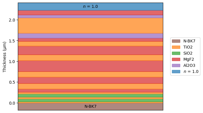
14. Dichroic spectral performance

The final comparison shows the starting (HL)³ stack vs. the optimized dichroic. The algorithm built a sharp transition edge at 550 nm using all four candidate materials.

# Rebuild starting design for comparison
stack_d_initial = ThinFilmStack(incident_material=air, substrate_material=nbk7)
for _ in range(3):
    stack_d_initial.add_layer_nm(tio2, 47.0, name="TiO2")
    stack_d_initial.add_layer_nm(sio2, 86.0, name="SiO2")

wl_eval = np.linspace(390, 730, 400)
R_d_initial = np.array([ThinFilmOperand.reflectance(stack_d_initial, wl) for wl in wl_eval])
R_d_final = np.array([ThinFilmOperand.reflectance(result_d.stack, wl) for wl in wl_eval])

fig, ax = plt.subplots(figsize=(9, 5))
ax.plot(wl_eval, R_d_initial * 100, "--", color="gray",
        linewidth=1.5, label="Starting design (6 layers)")
ax.plot(wl_eval, R_d_final * 100, "-", color="steelblue",
        linewidth=2, label=f"After needle synthesis ({len(result_d.stack.layers)} layers)")
ax.axvspan(420, 540, alpha=0.06, color="blue")
ax.axvspan(560, 680, alpha=0.06, color="red")
ax.axhline(95, color="blue", linestyle=":", linewidth=1, alpha=0.5, label="R > 95% spec")
ax.axhline(5, color="red", linestyle=":", linewidth=1, alpha=0.5, label="R < 5% spec")
ax.set_xlabel("Wavelength (nm)")
ax.set_ylabel("Reflectance (%)")
ax.set_title("Dichroic Beamsplitter on N-BK7 — Needle Synthesis Result")
ax.set_ylim(0, 100)
ax.legend(loc="center right")
ax.grid(True, alpha=0.3)
fig.tight_layout();