Tutorial 4d: Lens Catalogue Integration

Consolidating off-the-shelf catalog lens selection from Edmund Optics and Thorlabs catalogs.

This tutorial shows how to retrieve optical components from the Edmund Optics lens catalogue. In particular, we cover:

• How to open Zemax files in Optiland

• How to retrieve and analyze an aspheric lens from the Edmund Optics catalogue

Optiland uses the function load_zemax_file to load a Zemax (.zmx) files into the Optiland format. The function accepts either a file directly or a URL link to the file. If a URL is provided, Optiland downloads the file prior to extracting the lens data.

from optiland import analysis
from optiland.fileio import load_zemax_file

File retrieval

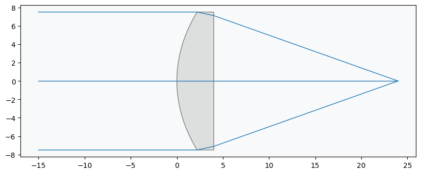
For this example, we will use a 15 mm Dia., 0.33 Numerical Aperture Uncoated, Aspheric Lens. We pass the filename of the downloaded .zmx file to our load_zemax_file function:

filename = "zmax_47728.zmx"  # downloaded from link above
lens = load_zemax_file(filename)

The function directly returns an instance of an Optiland Optic class. We can draw the lens as shown.

lens.draw()

We also print an overview of the lens data. This currently excludes the aspheric coefficients.

lens.info()

+----+---------------------+----------+-------------+------------+----------+-----------------+
|    | Type                |   Radius |   Thickness | Material   |    Conic |   Semi-aperture |
|----+---------------------+----------+-------------+------------+----------+-----------------|
|  0 | Planar              |  inf     |    inf      | Air        |  0       |     7.5         |
|  1 | Stop - Even Asphere |   13.255 |      4      | L-BAL35    | -2.36414 |     7.5         |
|  2 | Planar              |  inf     |     19.9823 | Air        |  0       |     6.66094     |
|  3 | Planar              |  inf     |    nan      | Air        |  0       |     2.66454e-15 |
+----+---------------------+----------+-------------+------------+----------+-----------------+

Lens Analysis

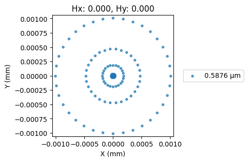
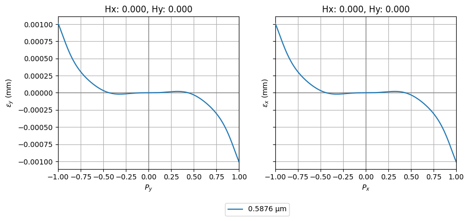
To assess performance, we generate a spot diagram and the ray aberration fans:

spot = analysis.SpotDiagram(lens)
spot.view()

fan = analysis.RayFan(lens)
fan.view()

Conclusions

• This tutorial showed how to retrieve and analyze an Edmund Optics catalogue lens.

• The load_zemax_file function does not currently support all Zemax surface types and may fail to convert a lens into an Optiland Optic instance in some cases. Users are encouraged to create an issue on the GitHub page if an error occurs.

---

Part 2: Thorlabs Catalogue

This tutorial shows how to retrieve optical components from the Thorlabs lens catalogue. Building on the previous tutorial, we will show:

• How to retrieve a lens model directly from the Thorlabs website

• How to modify the lens properties after retrieval

import matplotlib.pyplot as plt
import numpy as np

from optiland import analysis
from optiland.fileio import load_zemax_file

File retrieval

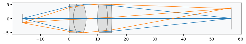
As mentioned in the previous tutorial, the load_zemax_file function can accept either a Zemax (.zmx) file directly or a URL link to the file. Here, we will use the a Thorlabs Matched Achromatic Pair Lens and we will pass the URL directly to ZemaxFileReader. Optiland will download the file prior to reading the .zmx file.

# link to the .zmx file on Thorlabs website
url = "https://www.thorlabs.com/_sd.cfm?fileName=20565-S03.zmx&partNumber=MAP051950-A"

lens = load_zemax_file(url)

We then draw the lens.

lens.draw()

Let’s print an overview of the lens data:

lens.info()

+----+---------------+----------+-------------+------------+---------+-----------------+
|    | Type          |   Radius |   Thickness | Material   |   Conic |   Semi-aperture |
|----+---------------+----------+-------------+------------+---------+-----------------|
|  0 | Planar        |   inf    |    16.3412  | Air        |       0 |        0.413735 |
|  1 | Standard      |    59.26 |     1.5     | N-SF6HT    |       0 |        4.633    |
|  2 | Standard      |    11.04 |     4.5     | N-BAF10    |       0 |        4.73714  |
|  3 | Standard      |   -12.94 |     2       | Air        |       0 |        5.23109  |
|  4 | Stop - Planar |   inf    |     1.98331 | Air        |       0 |        5.05599  |
|  5 | Standard      |    27.36 |     3.5     | N-BK7      |       0 |        5.19763  |
|  6 | Standard      |   -22.54 |     1.5     | SF2        |       0 |        5.13588  |
|  7 | Standard      |   -91.83 |    41.7305  | Air        |       0 |        5.13866  |
|  8 | Planar        |   inf    |   nan       | Air        |       0 |        3.75398  |
+----+---------------+----------+-------------+------------+---------+-----------------+

Lens Analysis

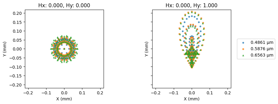
Let’s plot the nominal spot diagram:

spot = analysis.SpotDiagram(lens)
spot.view()

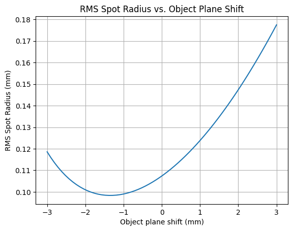
The lens is designed for finite conjugate applications. As an exercise, let’s monitor the RMS spot size as a function of the object position. As we shift the object plane, we will reposition the image plane to the paraxial image location. We will use the on-axis field point (index=0) and the central wavelength (index=1).

# we will shift the object plane by ±3.0 mm from the nominal location
dz = np.linspace(-3.0, 3.0, 64)

# thickness between the object surface and the first lens surface
thickness = dz + 16.3412  # nominal location = 16.3412 mm

# set the wavelength and field indices
wavelength_idx = 1
field_idx = 0

# initialize variables
rms_spot_radius = []

for z in thickness:
    # change thickness on the first surface
    lens.updater.set_thickness(value=z, surface_number=0)

    # move image plane to maintain focus
    lens.image_solve()

    # generate spot diagram data
    spot = analysis.SpotDiagram(lens)

    # calculate RMS spot radius
    rms_spot_radius.append(spot.rms_spot_radius()[field_idx][wavelength_idx])

plt.plot(dz, rms_spot_radius)
plt.xlabel("Object plane shift (mm)")
plt.ylabel("RMS Spot Radius (mm)")
plt.title("RMS Spot Radius vs. Object Plane Shift")
plt.grid()
plt.show()

Conclusions

• This tutorial showed how to retrieve and analyze a Thorlabs catalogue lens.

• We modified the lens properties and assessed the RMS spot size of the on-axis field as a function of the object plane shift. We compensated for the object shift by repositioning the image plane to the paraxial image location.