Tutorial 2d: OPD, PSF and MTF Calculations
Consolidating Optical Path Difference (OPD), Point Spread Function (PSF), Modulation Transfer Function (MTF), and Zernike decomposition wavefront fitting.
This tutorial demonstrates how to compute the optical path difference in the exit pupil and the various ways to plot it.
[1]:
from optiland import wavefront
from optiland.samples.eyepieces import EyepieceErfle
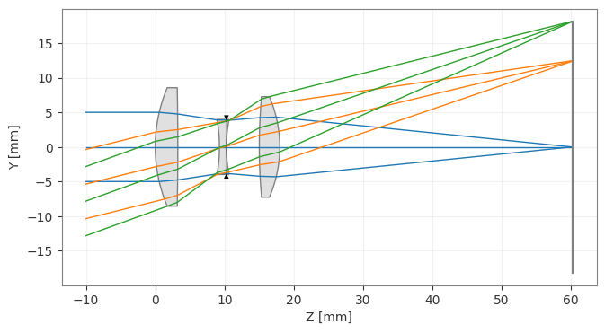
[2]:
lens = EyepieceErfle()
lens.draw()
[2]:
(<Figure size 1000x400 with 1 Axes>, <Axes: xlabel='Z [mm]', ylabel='Y [mm]'>)

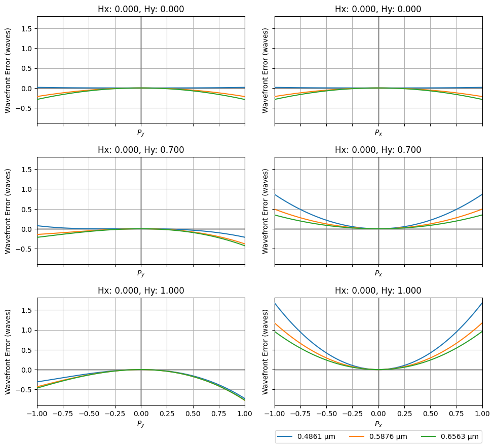
First, we compute the OPD fans for each field and wavelength.
[3]:
opd_fan = wavefront.OPDFan(lens)
opd_fan.view()
[3]:
(<Figure size 1000x900 with 6 Axes>,
 array([[<Axes: title={'center': 'Hx: 0.000, Hy: 0.000'}, xlabel='$P_y$', ylabel='Wavefront Error (waves)'>,
         <Axes: title={'center': 'Hx: 0.000, Hy: 0.000'}, xlabel='$P_x$', ylabel='Wavefront Error (waves)'>],
        [<Axes: title={'center': 'Hx: 0.000, Hy: 0.700'}, xlabel='$P_y$', ylabel='Wavefront Error (waves)'>,
         <Axes: title={'center': 'Hx: 0.000, Hy: 0.700'}, xlabel='$P_x$', ylabel='Wavefront Error (waves)'>],
        [<Axes: title={'center': 'Hx: 0.000, Hy: 1.000'}, xlabel='$P_y$', ylabel='Wavefront Error (waves)'>,
         <Axes: title={'center': 'Hx: 0.000, Hy: 1.000'}, xlabel='$P_x$', ylabel='Wavefront Error (waves)'>]],
       dtype=object))
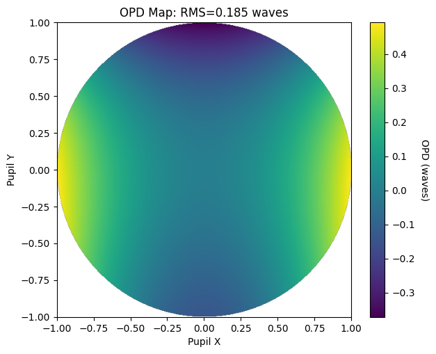
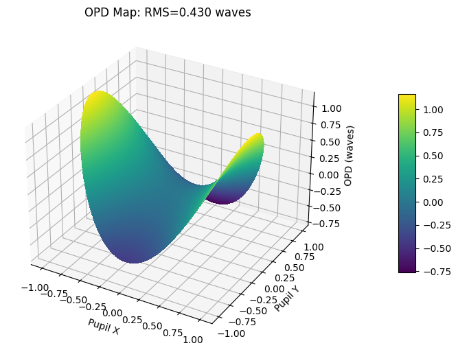
Next, we compute the wavefront map for each field and demonstrate different ways of plotting.
[4]:
opd = wavefront.OPD(lens, field=(0, 0), wavelength=0.5876)
opd.view(projection="2d", num_points=512)
[4]:
(<Figure size 700x550 with 2 Axes>,
 <Axes: title={'center': 'OPD Map: RMS=0.134 waves'}, xlabel='Pupil X', ylabel='Pupil Y'>)

[5]:
opd = wavefront.OPD(lens, field=(0, 0.7), wavelength=0.5876)
opd.view(projection="2d", num_points=512)
[5]:
(<Figure size 700x550 with 2 Axes>,
 <Axes: title={'center': 'OPD Map: RMS=0.185 waves'}, xlabel='Pupil X', ylabel='Pupil Y'>)
[6]:
opd = wavefront.OPD(lens, field=(0, 1.0), wavelength=0.5876)
opd.view(projection="3d", num_points=512)
[6]:
(<Figure size 700x550 with 2 Axes>,
 <Axes3D: title={'center': 'OPD Map: RMS=0.430 waves'}, xlabel='Pupil X', ylabel='Pupil Y', zlabel='OPD (waves)'>)
Part 2: PSF & MTF Calculation
This tutorial shows how to calculate the point spread function (PSF) and modulation transfer function (MTF) of a lens.
[1]:
from optiland import mtf, psf
from optiland.samples.objectives import CookeTriplet
[2]:
lens = CookeTriplet()
lens.draw()
[2]:
(<Figure size 1000x400 with 1 Axes>, <Axes: xlabel='Z [mm]', ylabel='Y [mm]'>)
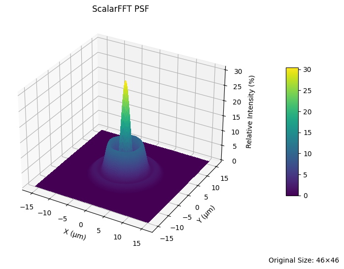
We first compute the PSF using the FFT-based approach. We demonstrate various ways to generate and plot the PSF.
[3]:
lens_psf = psf.FFTPSF(lens, field=(0, 0), wavelength=0.55)
lens_psf.view(projection="3d", num_points=256)
C:\Users\kdani\AppData\Local\Temp\ipykernel_30580\3512864652.py:2: UserWarning: The PSF view has a high oversampling factor (5.57). Results may be inaccurate.
  lens_psf.view(projection="3d", num_points=256)
[3]:
(<Figure size 700x550 with 2 Axes>,
 <Axes3D: title={'center': 'ScalarFFT PSF'}, xlabel='X (µm)', ylabel='Y (µm)', zlabel='Relative Intensity (%)'>)
[4]:
print(f"Strehl Ratio: {lens_psf.strehl_ratio():.3f}")
Strehl Ratio: 0.306
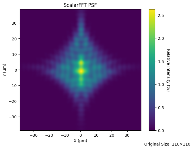
[5]:
lens_psf = psf.FFTPSF(lens, field=(0, 0.7), wavelength=0.55)
lens_psf.view(num_points=512)
C:\Users\kdani\AppData\Local\Temp\ipykernel_30580\3051880103.py:2: UserWarning: The PSF view has a high oversampling factor (4.65). Results may be inaccurate.
  lens_psf.view(num_points=512)
[5]:
(<Figure size 700x550 with 2 Axes>,
 <Axes: title={'center': 'ScalarFFT PSF'}, xlabel='X (µm)', ylabel='Y (µm)'>)
[6]:
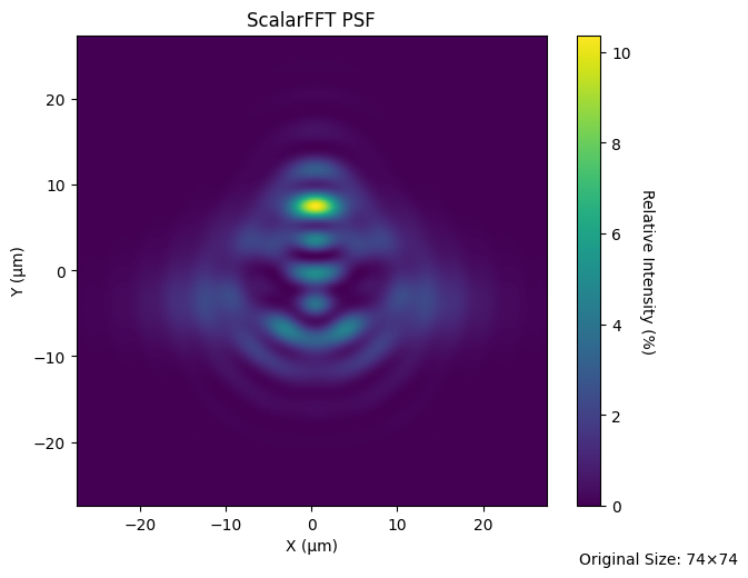
lens_psf = psf.FFTPSF(lens, field=(0, 1.0), wavelength=0.55)
lens_psf.view(projection="2d", num_points=256)
C:\Users\kdani\AppData\Local\Temp\ipykernel_30580\48181633.py:2: UserWarning: The PSF view has a high oversampling factor (3.46). Results may be inaccurate.
  lens_psf.view(projection="2d", num_points=256)
[6]:
(<Figure size 700x550 with 2 Axes>,
 <Axes: title={'center': 'ScalarFFT PSF'}, xlabel='X (µm)', ylabel='Y (µm)'>)
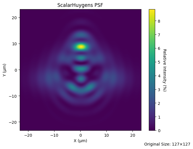
We can also generate the PSF using direct Huygens-Fresnel integration. This is referred to as the “Huygens PSF”.
[7]:
lens_huygens_psf = psf.HuygensPSF(lens, field=(0, 1.0), wavelength=0.55)
lens_huygens_psf.view(projection="2d", num_points=256)
[7]:
(<Figure size 700x550 with 2 Axes>,
 <Axes: title={'center': 'ScalarHuygens PSF'}, xlabel='X (µm)', ylabel='Y (µm)'>)
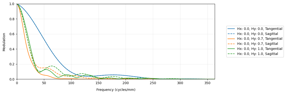
Now, we generate the geometric MTF, which uses only ray intersection locations on the image plane and ignores diffraction. The geometric MTF is a reasonable approximation when the lens is far from the diffraction limit.
As is standard, the geometric MTF is scaled based on the diffraction-limited MTF curve. This assures that the geometric MTF cannot show performance better than the diffraction limit.
[8]:
geo_mtf = mtf.GeometricMTF(lens)
geo_mtf.view()
[8]:
(<Figure size 1200x400 with 1 Axes>,
 <Axes: xlabel='Frequency (cycles/mm)', ylabel='Modulation'>)
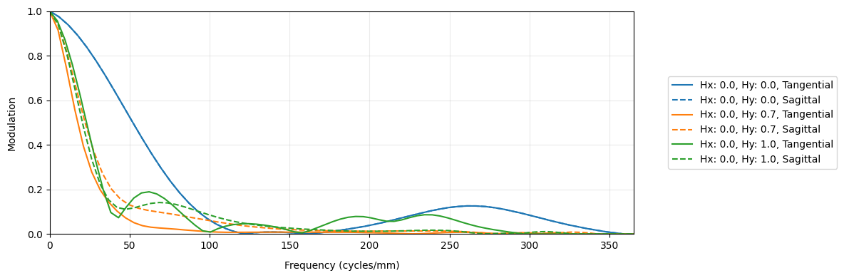
Finally, we show the standard FFT-based MTF.
[9]:
lens_mtf = mtf.FFTMTF(lens)
lens_mtf.view()
[9]:
(<Figure size 1200x400 with 1 Axes>,
 <Axes: xlabel='Frequency (cycles/mm)', ylabel='Modulation'>)
Part 3: Zernike Decomposition
This tutorial shows how to decompose the pupil using various Zernike types. Namely, we use “standard”, “fringe”, and “Noll” Zernike indices.
[1]:
import matplotlib.pyplot as plt

from optiland import wavefront
from optiland.samples.eyepieces import EyepieceErfle
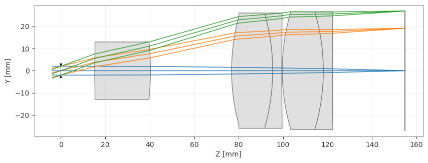
[2]:
lens = EyepieceErfle()
lens.draw()
[2]:
(<Figure size 1000x400 with 1 Axes>, <Axes: xlabel='Z [mm]', ylabel='Y [mm]'>)
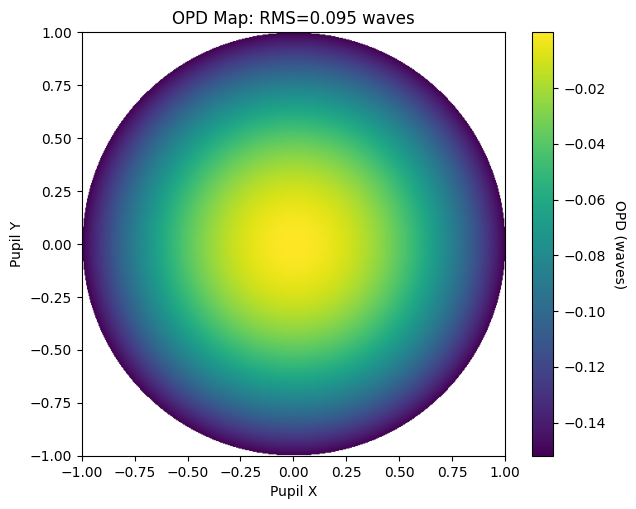
First, we’ll view the wavefront.
[3]:
opd = wavefront.OPD(lens, field=(0, 0), wavelength=0.55)
opd.view(projection="2d", num_points=512)
[3]:
(<Figure size 700x550 with 2 Axes>,
 <Axes: title={'center': 'OPD Map: RMS=0.095 waves'}, xlabel='Pupil X', ylabel='Pupil Y'>)
We’ll then find the Zernike coefficients of the wavefront.
[4]:
zernike_standard = wavefront.ZernikeOPD(
    lens,
    field=(0, 0),
    wavelength=0.55,
    zernike_type="standard",
    num_terms=37,
)
Let’s view the Zernike fit and compare it to the nominal OPD map.
[5]:
zernike_standard.view(projection="2d", num_points=512)
[5]:
(<Figure size 700x550 with 2 Axes>,
 <Axes: title={'center': 'Zernike Standard Fit'}, xlabel='Pupil X', ylabel='Pupil Y'>)
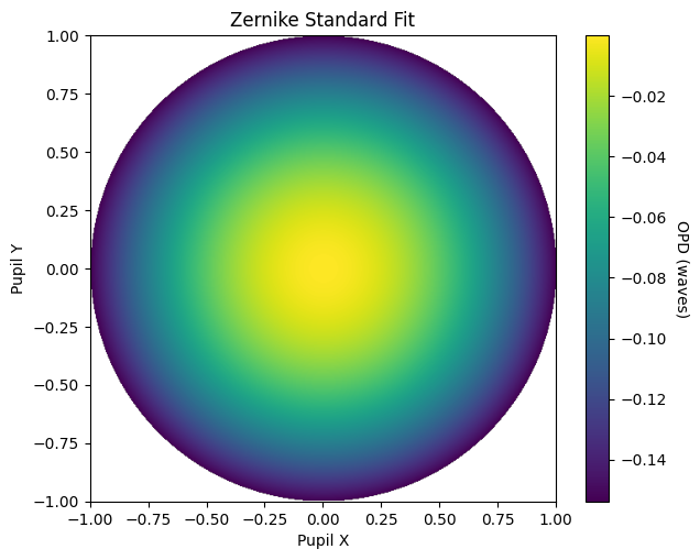
Qualitatively, we can see the Zernike fit well-represents the OPD map.
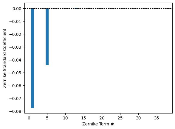
Let’s see what the actual coefficients look like:
[6]:
plt.bar(range(1, 38), zernike_standard.coeffs)
plt.axhline(color="k", linewidth=1, linestyle="--")
plt.xlabel("Zernike Term #")
plt.ylabel("Zernike Standard Coefficient")
plt.show()
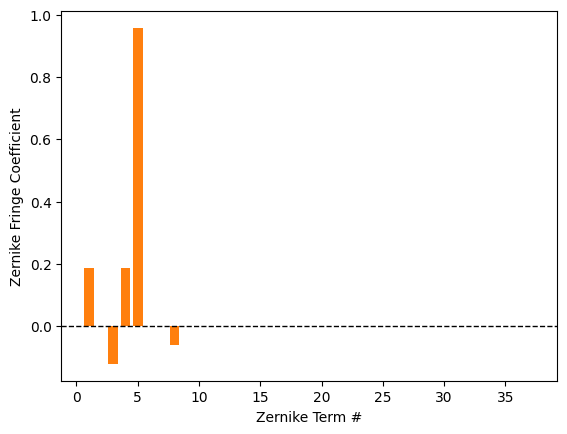
Let’s decompose the wavefront using Zernike fringe indices and Zernike Noll indices. We’ll use the field point at (0, 1).
[7]:
zernike_fringe = wavefront.ZernikeOPD(
    lens,
    field=(0, 1),
    wavelength=0.55,
    zernike_type="fringe",
    num_terms=37,
)

plt.bar(range(1, 38), zernike_fringe.coeffs, color="C1")
plt.axhline(color="k", linewidth=1, linestyle="--")
plt.xlabel("Zernike Term #")
plt.ylabel("Zernike Fringe Coefficient")
plt.show()
[8]:
zernike_noll = wavefront.ZernikeOPD(
    lens,
    field=(0, 1),
    wavelength=0.55,
    zernike_type="noll",
    num_terms=37,
)

plt.bar(range(1, 38), zernike_noll.coeffs, color="C2")
plt.axhline(color="k", linewidth=1, linestyle="--")
plt.xlabel("Zernike Term #")
plt.ylabel("Zernike Noll Coefficient")
plt.show()
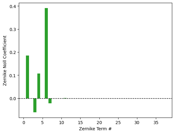
Or, if we just want to read off the coefficients, we can print them. Let’s only use 9 terms in this case:
[9]:
zernike = wavefront.ZernikeOPD(lens, (0, 1), 0.55, zernike_type="noll", num_terms=9)

for k in range(len(zernike.coeffs)):
    print(f"Z{k + 1}: {zernike.coeffs[k]:.8f}")
Z1: 0.18585891
Z2: -0.00000000
Z3: -0.06086925
Z4: 0.10781267
Z5: 0.00000000
Z6: 0.39115859
Z7: -0.02152073
Z8: -0.00000000
Z9: 0.00002531