Tutorial 2c: Aberration Analyses
Consolidating spot diagrams, ray fans, wavefront errors, Seidel aberration coefficients, and chromatic aberrations.
This tutorial demonstrates the various aberration plots and analyses that can be performed in Optiland. Namely, we cover:
Spot diagrams
Ray fans
Y-Ybar plots
Distortion / Grid distortion plots
Field curvature plots
[1]:
from optiland import analysis
from optiland.samples.objectives import CookeTriplet
[2]:
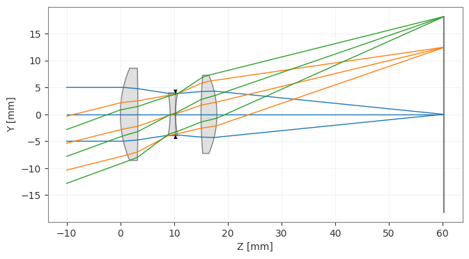
lens = CookeTriplet()
lens.draw()
[2]:
(<Figure size 1000x400 with 1 Axes>, <Axes: xlabel='Z [mm]', ylabel='Y [mm]'>)
Spot Diagram
[3]:
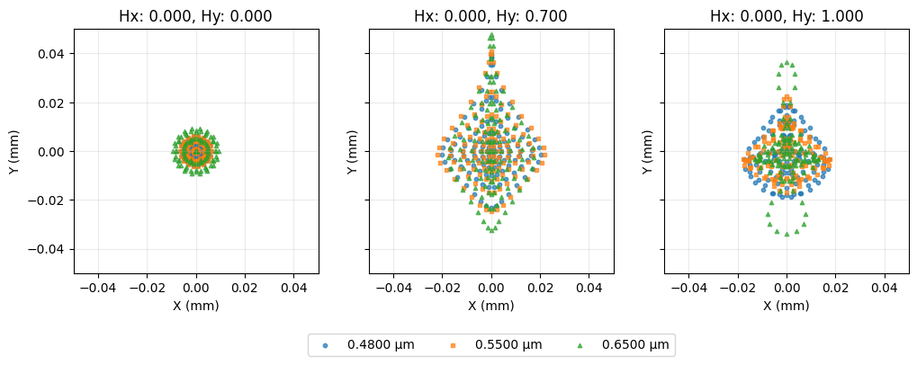
spot = analysis.SpotDiagram(lens)
spot.view()
[3]:
(<Figure size 1200x400 with 3 Axes>,
 [<Axes: title={'center': 'Hx: 0.000, Hy: 0.000'}, xlabel='X (mm)', ylabel='Y (mm)'>,
  <Axes: title={'center': 'Hx: 0.000, Hy: 0.700'}, xlabel='X (mm)', ylabel='Y (mm)'>,
  <Axes: title={'center': 'Hx: 0.000, Hy: 1.000'}, xlabel='X (mm)', ylabel='Y (mm)'>])
[4]:
fields = lens.fields.get_field_coords()
wavelengths = lens.wavelengths.get_wavelengths()
[5]:
print("Geometric Spot Radius:")

geo_spot_radius = spot.geometric_spot_radius()
for i, field in enumerate(fields):
    for j, wavelength in enumerate(wavelengths):
        print(
            f"\tField {field}, Wavelength {wavelength:.3f} µm, "
            f"Radius: {geo_spot_radius[i][j]:.5f} mm",
        )
Geometric Spot Radius:
        Field (0.0, 0.0), Wavelength 0.480 µm, Radius: 0.00597 mm
        Field (0.0, 0.0), Wavelength 0.550 µm, Radius: 0.00629 mm
        Field (0.0, 0.0), Wavelength 0.650 µm, Radius: 0.00932 mm
        Field (0.0, 0.7), Wavelength 0.480 µm, Radius: 0.03928 mm
        Field (0.0, 0.7), Wavelength 0.550 µm, Radius: 0.04075 mm
        Field (0.0, 0.7), Wavelength 0.650 µm, Radius: 0.04772 mm
        Field (0.0, 1.0), Wavelength 0.480 µm, Radius: 0.01891 mm
        Field (0.0, 1.0), Wavelength 0.550 µm, Radius: 0.02250 mm
        Field (0.0, 1.0), Wavelength 0.650 µm, Radius: 0.03655 mm
[6]:
print("RMS Spot Radius:")

rms_spot_radius = spot.rms_spot_radius()
for i, field in enumerate(fields):
    for j, wavelength in enumerate(wavelengths):
        print(
            f"\tField {field}, Wavelength {wavelength:.3f} µm, "
            f"Radius: {rms_spot_radius[i][j]:.5f} mm",
        )
RMS Spot Radius:
        Field (0.0, 0.0), Wavelength 0.480 µm, Radius: 0.00379 mm
        Field (0.0, 0.0), Wavelength 0.550 µm, Radius: 0.00429 mm
        Field (0.0, 0.0), Wavelength 0.650 µm, Radius: 0.00620 mm
        Field (0.0, 0.7), Wavelength 0.480 µm, Radius: 0.01582 mm
        Field (0.0, 0.7), Wavelength 0.550 µm, Radius: 0.01692 mm
        Field (0.0, 0.7), Wavelength 0.650 µm, Radius: 0.01922 mm
        Field (0.0, 1.0), Wavelength 0.480 µm, Radius: 0.01324 mm
        Field (0.0, 1.0), Wavelength 0.550 µm, Radius: 0.01212 mm
        Field (0.0, 1.0), Wavelength 0.650 µm, Radius: 0.01365 mm
Ray fans
[7]:
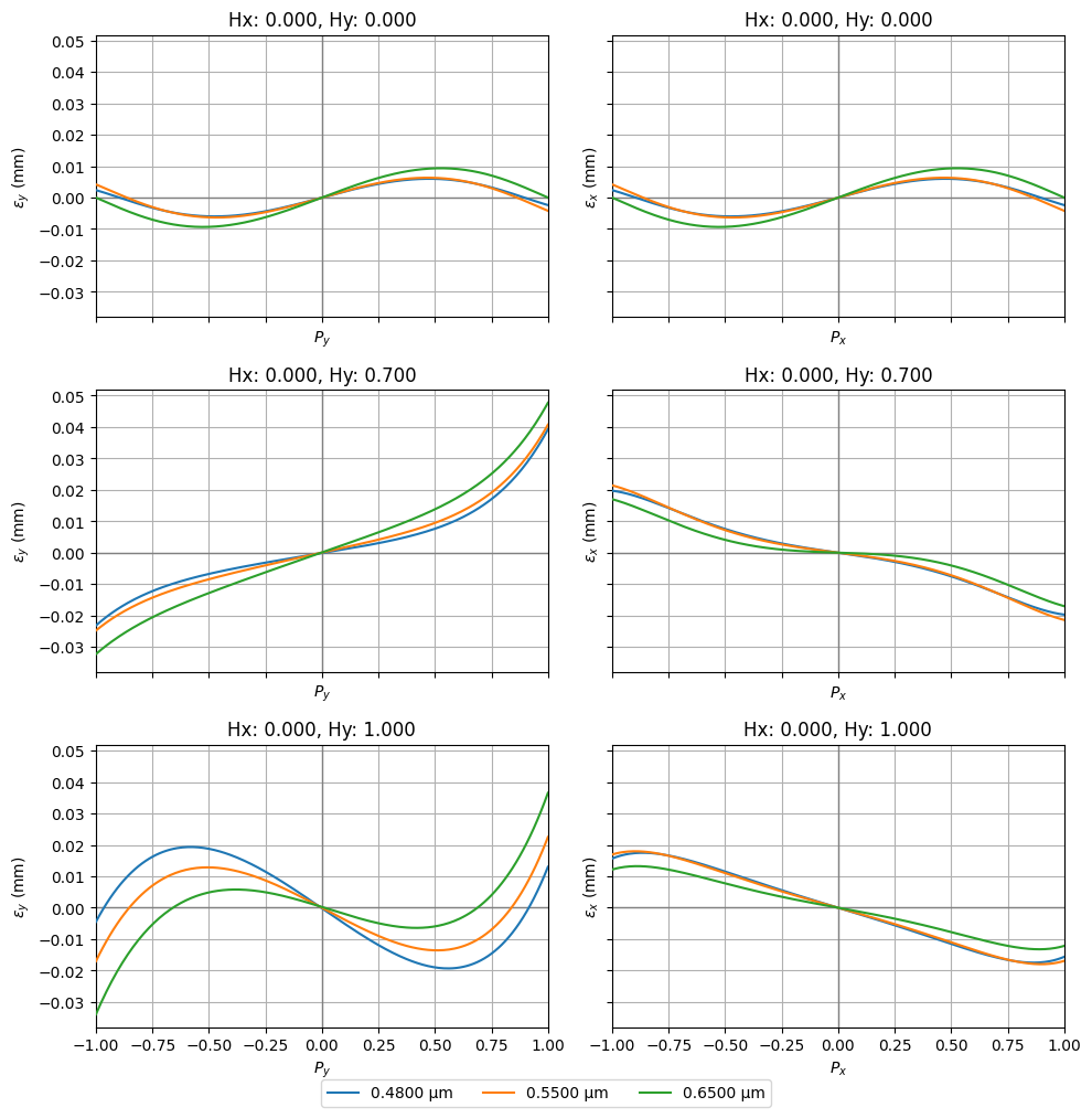
fan = analysis.RayFan(lens)
fan.view()
[7]:
(<Figure size 1000x999 with 6 Axes>,
 [<Axes: title={'center': 'Hx: 0.000, Hy: 0.000'}, xlabel='$P_y$', ylabel='$\\epsilon_y$ (mm)'>,
  <Axes: title={'center': 'Hx: 0.000, Hy: 0.000'}, xlabel='$P_x$', ylabel='$\\epsilon_x$ (mm)'>,
  <Axes: title={'center': 'Hx: 0.000, Hy: 0.700'}, xlabel='$P_y$', ylabel='$\\epsilon_y$ (mm)'>,
  <Axes: title={'center': 'Hx: 0.000, Hy: 0.700'}, xlabel='$P_x$', ylabel='$\\epsilon_x$ (mm)'>,
  <Axes: title={'center': 'Hx: 0.000, Hy: 1.000'}, xlabel='$P_y$', ylabel='$\\epsilon_y$ (mm)'>,
  <Axes: title={'center': 'Hx: 0.000, Hy: 1.000'}, xlabel='$P_x$', ylabel='$\\epsilon_x$ (mm)'>])
Y-Ybar plot
[8]:
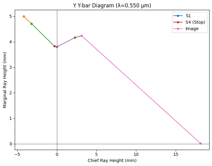
yybar = analysis.YYbar(lens)
yybar.view()
[8]:
(<Figure size 700x550 with 1 Axes>,
 <Axes: title={'center': 'Y Y-bar Diagram (λ=0.550 µm)'}, xlabel='Chief Ray Height (mm)', ylabel='Marginal Ray Height (mm)'>)
Distortion
[9]:
distortion = analysis.Distortion(lens)
distortion.view()
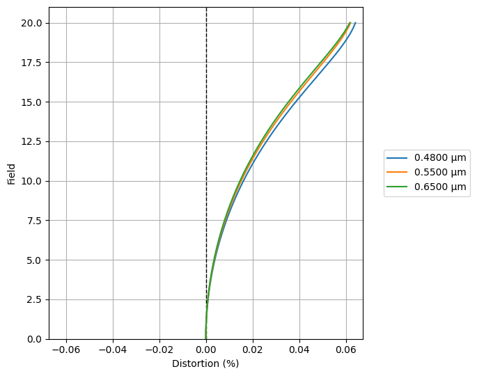
[9]:
(<Figure size 700x550 with 1 Axes>,
 <Axes: xlabel='Distortion (%)', ylabel='Field'>)
Grid distortion
[10]:
grid = analysis.GridDistortion(lens)
grid.view()
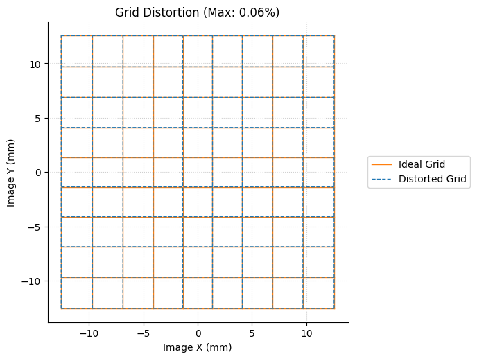
[10]:
(<Figure size 700x700 with 1 Axes>,
 <Axes: title={'center': 'Grid Distortion (Max: 0.06%)'}, xlabel='Image X (mm)', ylabel='Image Y (mm)'>)
Field Curvature
[11]:
field_curv = analysis.FieldCurvature(lens)
field_curv.view()
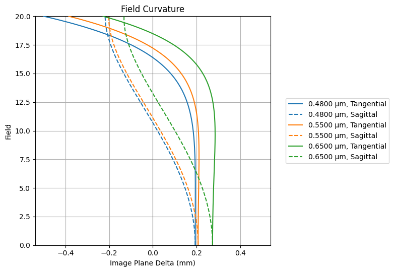
[11]:
(<Figure size 800x550 with 1 Axes>,
 <Axes: title={'center': 'Field Curvature'}, xlabel='Image Plane Delta (mm)', ylabel='Field'>)
RMS Spot Size vs. Field
[12]:
rms_spot_vs_field = analysis.RmsSpotSizeVsField(lens)
rms_spot_vs_field.view()
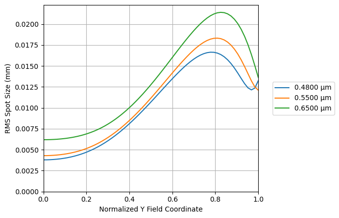
[12]:
(<Figure size 700x450 with 1 Axes>,
 <Axes: xlabel='Normalized Y Field Coordinate', ylabel='RMS Spot Size (mm)'>)
RMS Wavefront Error vs. Field
[13]:
rms_wavefront_error_vs_field = analysis.RmsWavefrontErrorVsField(lens)
rms_wavefront_error_vs_field.view()
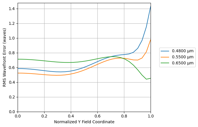
[13]:
(<Figure size 700x450 with 1 Axes>,
 <Axes: xlabel='Normalized Y Field Coordinate', ylabel='RMS Wavefront Error (waves)'>)
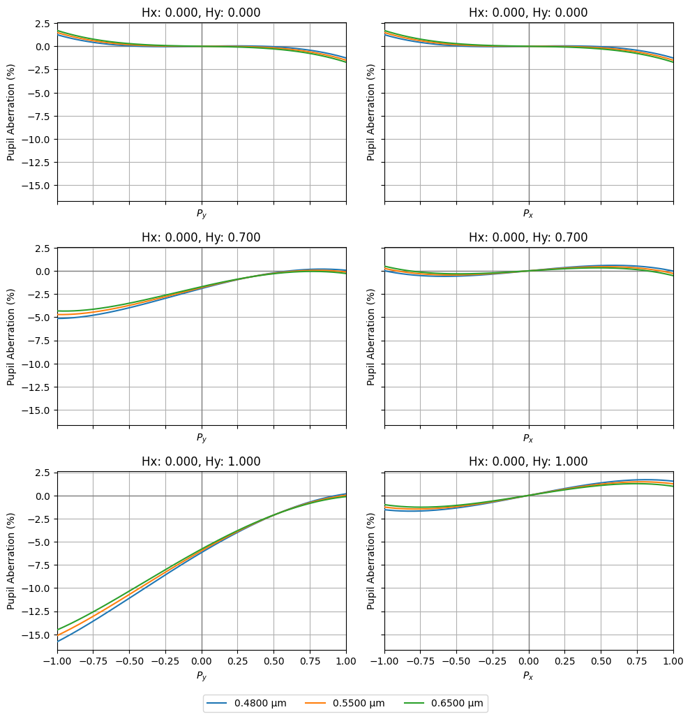
Pupil Aberration
The pupil abberration is defined as the difference between the paraxial and real ray intersection point at the stop surface of the optic. This is specified as a percentage of the on-axis paraxial stop radius at the primary wavelength.
[14]:
pupil_ab = analysis.PupilAberration(lens)
pupil_ab.view()
[14]:
(<Figure size 1000x999 with 6 Axes>,
 array([[<Axes: title={'center': 'Hx: 0.000, Hy: 0.000'}, xlabel='$P_y$', ylabel='Pupil Aberration (%)'>,
         <Axes: title={'center': 'Hx: 0.000, Hy: 0.000'}, xlabel='$P_x$', ylabel='Pupil Aberration (%)'>],
        [<Axes: title={'center': 'Hx: 0.000, Hy: 0.700'}, xlabel='$P_y$', ylabel='Pupil Aberration (%)'>,
         <Axes: title={'center': 'Hx: 0.000, Hy: 0.700'}, xlabel='$P_x$', ylabel='Pupil Aberration (%)'>],
        [<Axes: title={'center': 'Hx: 0.000, Hy: 1.000'}, xlabel='$P_y$', ylabel='Pupil Aberration (%)'>,
         <Axes: title={'center': 'Hx: 0.000, Hy: 1.000'}, xlabel='$P_x$', ylabel='Pupil Aberration (%)'>]],
       dtype=object))
Part 2: First & Third Order Aberrations
This tutorial illustrates how various aberration coefficients are computed.
[15]:
from optiland.samples.objectives import TripletTelescopeObjective
[16]:
lens = TripletTelescopeObjective()
lens.draw()
[16]:
(<Figure size 1000x400 with 1 Axes>, <Axes: xlabel='Z [mm]', ylabel='Y [mm]'>)
[17]:
print("Seidel Aberrations:")
for k, seidel in enumerate(lens.aberrations.seidels()):
    print(f"\tS{k + 1}: {seidel:.3e}")
Seidel Aberrations:
        S1: -2.707e-03
        S2: -1.412e-03
        S3: -1.479e-03
        S4: -5.568e-04
        S5: 3.606e-05
[18]:
print("Third-order transverse spherical aberration:")
for k, value in enumerate(lens.aberrations.TSC()):
    print(f"\tSurface {k + 1}: {value:.3e}")
Third-order transverse spherical aberration:
        Surface 1: -5.087e-01
        Surface 2: -2.442e-01
        Surface 3: 2.466e-02
        Surface 4: -2.759e+00
        Surface 5: 3.481e+00
        Surface 6: -5.623e-04
[19]:
print("Third-order longitudinal spherical aberration:")
for k, value in enumerate(lens.aberrations.SC()):
    print(f"\tSurface {k + 1}: {value:.3e}")
Third-order longitudinal spherical aberration:
        Surface 1: -2.849e+00
        Surface 2: -1.367e+00
        Surface 3: 1.381e-01
        Surface 4: -1.545e+01
        Surface 5: 1.949e+01
        Surface 6: -3.149e-03
[20]:
print("Third-order sagittal coma:")
for k, value in enumerate(lens.aberrations.CC()):
    print(f"\tSurface {k + 1}: {value:.3e}")
Third-order sagittal coma:
        Surface 1: -2.491e-02
        Surface 2: 2.011e-02
        Surface 3: 4.053e-03
        Surface 4: 8.930e-02
        Surface 5: -9.345e-02
        Surface 6: 9.330e-04
[21]:
print("Third-order tangential coma:")
for k, value in enumerate(lens.aberrations.TCC()):
    print(f"\tSurface {k + 1}: {value:.3e}")
Third-order tangential coma:
        Surface 1: -7.473e-02
        Surface 2: 6.034e-02
        Surface 3: 1.216e-02
        Surface 4: 2.679e-01
        Surface 5: -2.803e-01
        Surface 6: 2.799e-03
[22]:
print("Third-order transverse astigmatism:")
for k, value in enumerate(lens.aberrations.TAC()):
    print(f"\tSurface {k + 1}: {value:.3e}")
Third-order transverse astigmatism:
        Surface 1: -1.220e-03
        Surface 2: -1.657e-03
        Surface 3: 6.659e-04
        Surface 4: -2.890e-03
        Surface 5: 2.509e-03
        Surface 6: -1.548e-03
[23]:
print("Third-order longitudinal astigmatism:")
for k, value in enumerate(lens.aberrations.AC()):
    print(f"\tSurface {k + 1}: {value:.3e}")
Third-order longitudinal astigmatism:
        Surface 1: -6.831e-03
        Surface 2: -9.280e-03
        Surface 3: 3.729e-03
        Surface 4: -1.618e-02
        Surface 5: 1.405e-02
        Surface 6: -8.670e-03
[24]:
print("Third-order transverse Petzval sum:")
for k, value in enumerate(lens.aberrations.TPC()):
    print(f"\tSurface {k + 1}: {value:.3e}")
Third-order transverse Petzval sum:
        Surface 1: -1.850e-03
        Surface 2: -9.425e-05
        Surface 3: -1.636e-03
        Surface 4: -5.416e-04
        Surface 5: 1.167e-03
        Surface 6: 1.395e-03
[25]:
print("Third-order longitudinal Petzval sum:")
for k, value in enumerate(lens.aberrations.PC()):
    print(f"\tSurface {k + 1}: {value:.3e}")
Third-order longitudinal Petzval sum:
        Surface 1: -1.036e-02
        Surface 2: -5.278e-04
        Surface 3: -9.159e-03
        Surface 4: -3.033e-03
        Surface 5: 6.537e-03
        Surface 6: 7.812e-03
[26]:
print("Third-order distortion:")
for k, value in enumerate(lens.aberrations.DC()):
    print(f"\tSurface {k + 1}: {value:.3e}")
Third-order distortion:
        Surface 1: -1.503e-04
        Surface 2: 1.443e-04
        Surface 3: -1.593e-04
        Surface 4: 1.111e-04
        Surface 5: -9.870e-05
        Surface 6: 2.540e-04
[27]:
print("First-order transverse axial color:")
for k, value in enumerate(lens.aberrations.TAchC()):
    print(f"\tSurface {k + 1}: {value:.3e}")
First-order transverse axial color:
        Surface 1: -1.893e-01
        Surface 2: -1.120e-01
        Surface 3: -5.758e-02
        Surface 4: -2.546e-01
        Surface 5: 7.011e-01
        Surface 6: -1.541e-02
[28]:
print("First-order longitudinal axial color:")
for k, value in enumerate(lens.aberrations.LchC()):
    print(f"\tSurface {k + 1}: {value:.3e}")
First-order longitudinal axial color:
        Surface 1: -1.060e+00
        Surface 2: -6.274e-01
        Surface 3: -3.224e-01
        Surface 4: -1.426e+00
        Surface 5: 3.926e+00
        Surface 6: -8.627e-02
[29]:
print("First-order lateral color:")
for k, value in enumerate(lens.aberrations.TchC()):
    print(f"\tSurface {k + 1}: {value:.3e}")
First-order lateral color:
        Surface 1: -9.272e-03
        Surface 2: 9.230e-03
        Surface 3: -9.461e-03
        Surface 4: 8.240e-03
        Surface 5: -1.882e-02
        Surface 6: 2.556e-02
Part 3: Chromatic Aberrations
This tutorial demonstrates how to assess chromatic aberrations in Optiland. We will first investigate a singlet with poor color correction, and then a well-corrected achromatic doublet.
[30]:
import numpy as np

from optiland import analysis, optic
Let’s define a simple singlet using a material with high dispersion:
[31]:
class Singlet(optic.Optic):
    """Simple Singlet"""

    def __init__(self):
        super().__init__()

        # add surfaces
        self.surfaces.add(index=0, radius=np.inf, thickness=np.inf)
        self.surfaces.add(
            index=1,
            thickness=0.5,
            radius=32.2526,
            is_stop=True,
            material="N-SF6",
        )
        self.surfaces.add(index=2, thickness=19.8532, radius=-31.9756)
        self.surfaces.add(index=3)

        # add aperture
        self.set_aperture(aperture_type="EPD", value=3.4)

        # add field
        self.fields.set_type(field_type="angle")
        self.fields.add(y=0.0)

        # add wavelength
        self.wavelengths.add(value=0.48613270)
        self.wavelengths.add(value=0.58756180, is_primary=True)
        self.wavelengths.add(value=0.65627250)
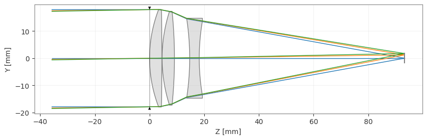
[32]:
singlet = Singlet()
singlet.draw(
    wavelengths=[0.48613270, 0.587561806, 0.65627250],
    figsize=(16, 4),
    num_rays=3,
)
[32]:
(<Figure size 1600x400 with 1 Axes>, <Axes: xlabel='Z [mm]', ylabel='Y [mm]'>)
As can be seen in the visualization, the wavelengths of light focus at different points on the optical axis (zooming in can also help to see this more clearly). To quantify this, let’s compute the first-order longitudinal axial color:
[33]:
print(f"First-order Longitudinal Color: {np.sum(singlet.aberrations.LchC()):.3f}")
First-order Longitudinal Color: -0.789
This can also be seen in ray aberration plots. The slope of the tranverse errors at the \(P_x=0\) and \(P_y=0\) locations vary with wavelength. This indicates that the defocus differs as a function of wavelength.
[34]:
fan = analysis.RayFan(singlet)
fan.view()
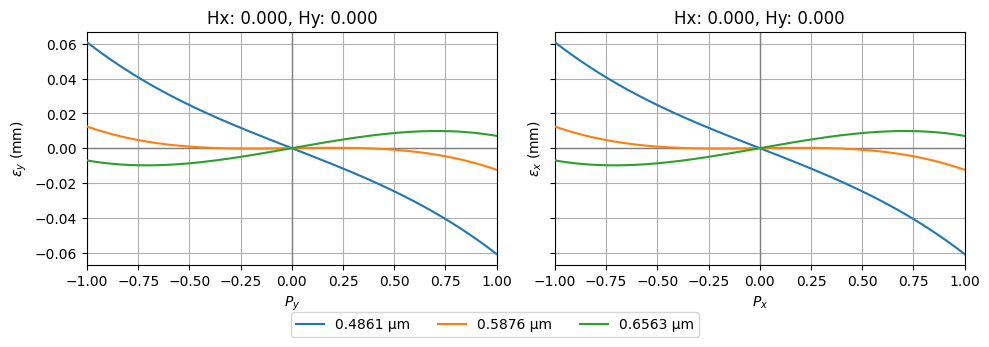
[34]:
(<Figure size 1000x333 with 2 Axes>,
 [<Axes: title={'center': 'Hx: 0.000, Hy: 0.000'}, xlabel='$P_y$', ylabel='$\\epsilon_y$ (mm)'>,
  <Axes: title={'center': 'Hx: 0.000, Hy: 0.000'}, xlabel='$P_x$', ylabel='$\\epsilon_x$ (mm)'>])
Now, let’s define an achromatic doublet, which improves the chromatic aberration performance in comparison to our simple singlet:
[35]:
class Doublet(optic.Optic):
    """Achromatic Doublet

    Milton Laikin, Lens Design, 4th ed., CRC Press, 2007, p. 45
    """

    def __init__(self):
        super().__init__()

        # add surfaces
        self.surfaces.add(index=0, radius=np.inf, thickness=np.inf)
        self.surfaces.add(
            index=1,
            radius=12.38401,
            thickness=0.4340,
            is_stop=True,
            material="N-BAK1",
        )
        self.surfaces.add(
            index=2,
            radius=-7.94140,
            thickness=0.3210,
            material=("SF2", "schott"),
        )
        self.surfaces.add(index=3, radius=-48.44396, thickness=19.6059)
        self.surfaces.add(index=4)

        # add aperture
        self.set_aperture(aperture_type="EPD", value=3.4)

        # add field
        self.fields.set_type(field_type="angle")
        self.fields.add(y=0)

        # add wavelength
        self.wavelengths.add(value=0.48613270)
        self.wavelengths.add(value=0.58756180, is_primary=True)
        self.wavelengths.add(value=0.65627250)
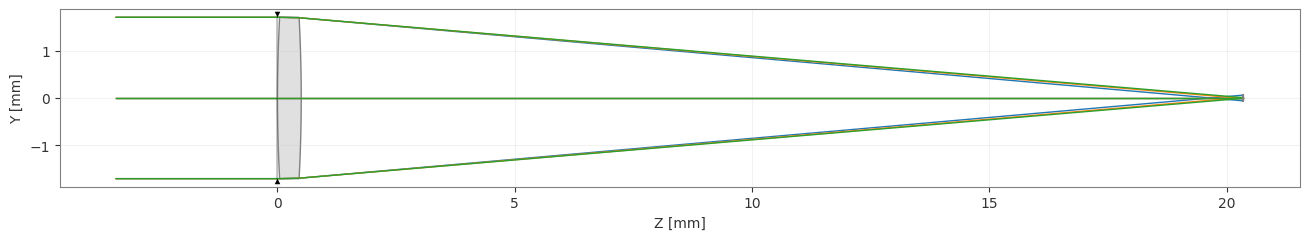
[36]:
doublet = Doublet()
doublet.draw(
    wavelengths=[0.48613270, 0.587561806, 0.65627250],
    figsize=(16, 4),
    num_rays=3,
)
[36]:
(<Figure size 1600x400 with 1 Axes>, <Axes: xlabel='Z [mm]', ylabel='Y [mm]'>)
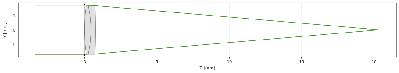
We can already see that the various wavelengths appear to focus at a similar location. Let’s confirm that the longitudinal chromatic aberration has indeed been reduced by computing this directly and generating the tranverse ray aberrations plots.
[37]:
print(f"First-order Longitudinal Color: {np.sum(doublet.aberrations.LchC()):.3f}")
First-order Longitudinal Color: -0.015
This value was -0.789 for the singlet and is now -0.015 for the doublet, which is a significant improvement. Now let’s look at the tranverse ray aberration plots:
[38]:
fan = analysis.RayFan(doublet)
fan.view()
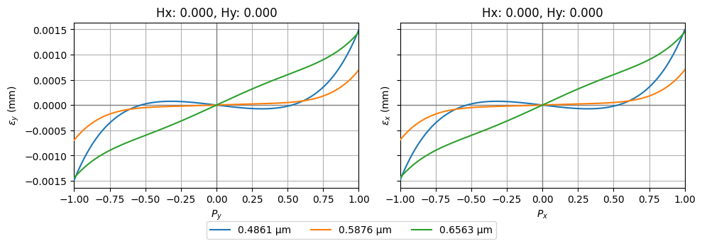
[38]:
(<Figure size 1000x333 with 2 Axes>,
 [<Axes: title={'center': 'Hx: 0.000, Hy: 0.000'}, xlabel='$P_y$', ylabel='$\\epsilon_y$ (mm)'>,
  <Axes: title={'center': 'Hx: 0.000, Hy: 0.000'}, xlabel='$P_x$', ylabel='$\\epsilon_x$ (mm)'>])
Note that the y-axis scale of this plot is significantly smaller than that of the singlet. We can confirm that chromatic aberrations have been significantly reduced.