Tutorial 1b: Lens Properties and Prescription Reports
Consolidating paraxial metrics, first-order calculations, and generating console and PDF prescription reports.
This tutorial describes how to retrieve common optical properties from a lens in Optiland, including:
Front and back focal length
Front and back, principle, focal, and nodal plane locations
Aperture information, such as F-Number, entrance or exit pupil diameter, etc.
Locations of entrance/exit pupils
Optical invariant
Marginal/chief rays
[1]:
from optiland.samples.objectives import CookeTriplet
[2]:
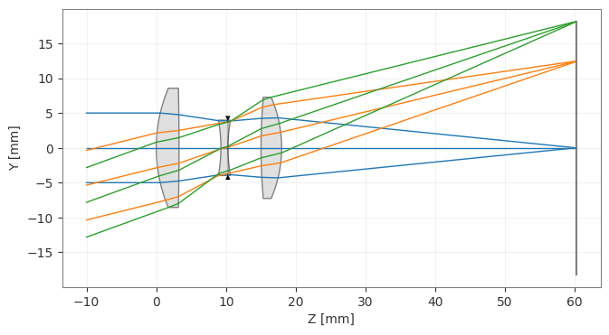
lens = CookeTriplet()
[3]:
lens.draw()
[3]:
(<Figure size 1000x400 with 1 Axes>, <Axes: xlabel='Z [mm]', ylabel='Y [mm]'>)
[4]:
print(f"Front focal length: {lens.paraxial.f1():.1f} mm")
print(f"Focal length: {lens.paraxial.f2():.1f} mm")
print(f"Front focal point: {lens.paraxial.F1():.1f} mm")
print(f"Back focal point: {lens.paraxial.F2():.1f} mm")
print(f"Front principal plane: {lens.paraxial.P1():.1f} mm")
print(f"Back principal plane: {lens.paraxial.P2():.1f} mm")
print(f"Front nodal plane: {lens.paraxial.N1():.1f} mm")
print(f"Back nodal plane: {lens.paraxial.N2():.1f} mm")
Front focal length: -50.0 mm
Focal length: 50.0 mm
Front focal point: -37.3 mm
Back focal point: 0.2 mm
Front principal plane: 12.7 mm
Back principal plane: -49.8 mm
Front nodal plane: 12.7 mm
Back nodal plane: -49.8 mm
Regarding cardinal points, Optiland defines object space quantities relative to the first lens surface (index 1) and image space quantities relative to the image surface. This applies to the pupil locations too: EPL() is relative to surface 1 and XPL() is relative to the image surface. If you need the entrance pupil as a global z coordinate, use lens.paraxial.entrance_pupil_z().
[5]:
print(f"Entrance pupil diameter: {lens.paraxial.EPD():.1f} mm")
print(f"Exit pupil diameter: {lens.paraxial.XPD():.1f} mm")
Entrance pupil diameter: 10.0 mm
Exit pupil diameter: 10.2 mm
[6]:
print(f"Entrance pupil position: {lens.paraxial.EPL():.1f} mm")
print(f"Exit pupil position: {lens.paraxial.XPL():.1f} mm")
Entrance pupil position: 11.5 mm
Exit pupil position: -51.0 mm
Magnification is generally computed for finite objects and not for systems like the one we’re analyzing here. We compute it only as an illustration.
[7]:
print(f"Image-space F-Number: {lens.paraxial.FNO():.1f}")
print(f"Magnification: {lens.paraxial.magnification():.1f}")
print(f"Invariant: {lens.paraxial.invariant():.3f}")
Image-space F-Number: 5.0
Magnification: -0.0
Invariant: -1.820
[8]:
print("Marginal Ray: ")

ya, ua = lens.paraxial.marginal_ray()
for k in range(len(ya)):
    print(f"\tSurface {k}: y = {ya[k, 0]:.3f}, u = {ua[k, 0]:.3f}")
Marginal Ray:
        Surface 0: y = 5.000, u = 0.000
        Surface 1: y = 5.000, u = -0.087
        Surface 2: y = 4.716, u = -0.148
        Surface 3: y = 3.826, u = -0.025
        Surface 4: y = 3.801, u = 0.076
        Surface 5: y = 4.162, u = 0.027
        Surface 6: y = 4.242, u = -0.100
        Surface 7: y = 0.021, u = -0.100
[9]:
print("Chief Ray: ")

yb, ub = lens.paraxial.chief_ray()
for k in range(len(yb)):
    print(f"\tSurface {k}: y = {yb[k, 0]:.3f}, u = {ub[k, 0]:.3f}")
Chief Ray:
        Surface 0: y = -4.190, u = 0.364
        Surface 1: y = -4.190, u = 0.297
        Surface 2: y = -3.221, u = 0.487
        Surface 3: y = -0.295, u = 0.295
        Surface 4: y = -0.000, u = 0.479
        Surface 5: y = 2.275, u = 0.284
        Surface 6: y = 3.113, u = 0.356
        Surface 7: y = 18.125, u = 0.356
Part 2: Prescription Generator
[1]:
from optiland.prescription import Prescription
from optiland.samples.objectives import CookeTriplet
1. What is a prescription?
A prescription summarises an optical system across five sections:
Section |
Contents |
|---|---|
System Overview |
Name, aperture type, fields, wavelengths |
First-Order Properties |
EFL, BFL, FFL, magnification, NAs, pupil positions |
Surface Geometry Table |
Radius, conic, thickness, aperture stop flag for every surface |
Surface Material Table |
Material name, nd, Abbe number, type for every surface |
Seidel Aberrations |
W040, W131, W222, W220, W311 and their totals |
2. Generating a prescription for a sample lens
Prescription(lens).view() prints a Rich-formatted table to the console. This requires the optional rich package (pip install rich).
[2]:
lens = CookeTriplet()

p = Prescription(lens)
p.view()
╭─────────────────────────────────────────────────────────────────────────────────────────────────────────────────╮
│ Optical Prescription — Unnamed System                                                                           │
╰──────────────────────────────────────── Generated: 2026-05-22 14:59 UTC ────────────────────────────────────────╯
───────────────────────────────────────────────── System Overview ─────────────────────────────────────────────────
  Name              (unnamed)
  Surfaces          6
  Stop Surface      4.0000
  Aperture Type     EPDAperture
  Aperture Value    10.0000
  Object Distance   ∞
  Image Distance    42.2078
Wavelengths
  #   Wavelength (µm)   Primary
 ━━━━━━━━━━━━━━━━━━━━━━━━━━━━━━━
  1   0.4800
  2   0.5500            ✓
  3   0.6500
Fields
  #   Type         X        Y         Weight
 ━━━━━━━━━━━━━━━━━━━━━━━━━━━━━━━━━━━━━━━━━━━━
  1   AngleField   0.0000   0.0000    1.0000
  2   AngleField   0.0000   14.0000   1.0000
  3   AngleField   0.0000   20.0000   1.0000
───────────────────────────────────────────── First-Order Properties ──────────────────────────────────────────────
  Effective Focal Length (EFL)   49.9998
  Front Focal Length (FFL)       -49.9998
  Back Focal Length (BFL)        0.2071
  Front Principal Plane (P1)     12.6541
  Back Principal Plane (P2)      -49.7927
  Front Nodal Plane (N1)         12.6541
  Back Nodal Plane (N2)          -49.7927
  Image-Space F/#                5.0000
  Entrance Pupil Diameter        10.0000
  Entrance Pupil Location        11.5122
  Exit Pupil Diameter            10.2337
  Exit Pupil Location            -50.9613
  Transverse Magnification       -0.0000
  Lagrange Invariant             -1.8199
───────────────────────────────────────────── Surface Data — Geometry ─────────────────────────────────────────────
  S#   Type       Radius (mm)   Thickness (mm)   Conic    Stop   Comment
 ━━━━━━━━━━━━━━━━━━━━━━━━━━━━━━━━━━━━━━━━━━━━━━━━━━━━━━━━━━━━━━━━━━━━━━━━
  0    Plane      ∞             ∞                —
  1    standard   22.0136       3.2590           0.0000
  2    standard   -435.7604     6.0076           0.0000
  3    standard   -22.2133      1.0000           0.0000
  4    standard   20.2919       4.7504           0.0000   ✓
  5    standard   79.6836       2.9521           0.0000
  6    standard   -18.3953      42.2078          0.0000
  7    standard   ∞             0.0000           —
──────────────────────────────────────────── Surface Data — Materials ─────────────────────────────────────────────
  S#   Material   nd       Vd        Semi-Diameter (mm)   Coating
 ━━━━━━━━━━━━━━━━━━━━━━━━━━━━━━━━━━━━━━━━━━━━━━━━━━━━━━━━━━━━━━━━━
  0    Air        1.0000   —         —                    —
  1    SK16       1.6204   60.2809   —                    —
  2    Air        1.0000   —         —                    —
  3    F2         1.6200   36.3665   —                    —
  4    Air        1.0000   —         —                    —
  5    SK16       1.6204   60.2809   —                    —
  6    Air        1.0000   —         —                    —
  7    Air        1.0000   —         —                    —
───────────────────────────────────────── Seidel Aberration Coefficients ──────────────────────────────────────────
  S#      SI (Sph)    SII (Coma)   SIII (Astig)   SIV (Petz)   SV (Dist)   CL (LCA)    CT (TCA)
 ━━━━━━━━━━━━━━━━━━━━━━━━━━━━━━━━━━━━━━━━━━━━━━━━━━━━━━━━━━━━━━━━━━━━━━━━━━━━━━━━━━━━━━━━━━━━━━━━
  1       -0.013855   -0.010591    -0.008096      -0.057727    -0.050318   -0.014412   -0.011017
  2       -0.011256   0.035011     -0.108897      -0.002916    0.347781    -0.010088   0.031376
  3       0.052115    -0.081389    0.127106       0.057268     -0.287939   0.031745    -0.049577
  4       0.024135    0.043874     0.079756       0.062690     0.258946    0.021172    0.038488
  5       -0.004080   -0.016132    -0.063784      -0.015948    -0.315255   -0.006189   -0.024472
  6       -0.054020   0.030462     -0.017178      -0.069082    0.048643    -0.017462   0.009847
  Total   -0.006960   0.001235     0.008907       -0.025716    0.001859    0.004767    -0.005356
3. Prescription output fields — the Document model
Prescription.build() returns a Document object without printing anything. You can inspect each section programmatically.
[3]:
doc = p.build()

print("Document title  :", doc.title)
print("Generated at    :", doc.generated_at)
print("Number of sections:", len(doc.sections))

for section in doc.sections:
    print(f"  Section: {section.title!r}")
Document title  : Optical Prescription — Unnamed System
Generated at    : 2026-05-22 14:59 UTC
Number of sections: 5
  Section: 'System Overview'
  Section: 'First-Order Properties'
  Section: 'Surface Data — Geometry'
  Section: 'Surface Data — Materials'
  Section: 'Seidel Aberration Coefficients'
[4]:
# Inspect the first-order properties section (KeyValueBlock rows)
first_order_section = doc.sections[1]
print(f"Section: {first_order_section.title}")
for block in first_order_section.blocks:
    if hasattr(block, "rows"):  # KeyValueBlock
        for label, value in block.rows:
            print(f"  {label}: {value}")
Section: First-Order Properties
  Effective Focal Length (EFL): 49.9998
  Front Focal Length (FFL): -49.9998
  Back Focal Length (BFL): 0.2071
  Front Principal Plane (P1): 12.6541
  Back Principal Plane (P2): -49.7927
  Front Nodal Plane (N1): 12.6541
  Back Nodal Plane (N2): -49.7927
  Image-Space F/#: 5.0000
  Entrance Pupil Diameter: 10.0000
  Entrance Pupil Location: 11.5122
  Exit Pupil Diameter: 10.2337
  Exit Pupil Location: -50.9613
  Transverse Magnification: -0.0000
  Lagrange Invariant: -1.8199
4. Saving to plain text
Prescription.save(path) infers the renderer from the file extension. Any extension other than .pdf produces a plain-text report.
[5]:
p.save("cooke_triplet.txt")

# Verify the file was written
with open("cooke_triplet.txt", "r", encoding="utf-8") as f:
    content = f.read()

print(content[:800])  # print first 800 characters
══════════════════════════════════════════════════════════════════════
  OPTICAL PRESCRIPTION — UNNAMED SYSTEM
  Generated: 2026-05-22 14:59 UTC
══════════════════════════════════════════════════════════════════════

┌─ System Overview ──────────────────────────────────────────────────┐
  Name              (unnamed)
  Surfaces          6
  Stop Surface      4.0000
  Aperture Type     EPDAperture
  Aperture Value    10.0000
  Object Distance   ∞
  Image Distance    42.2078

  Wavelengths
  #   Wavelength (µm)   Primary
  ─   ───────────────   ───────
  1   0.4800
  2   0.5500            ✓
  3   0.6500

  Fields
  #   Type         X        Y         Weight
  ─   ──────────   ──────   ───────   ──────
  1   AngleField   0.0000   0.0000    1.0000
  2
5. Exporting to PDF
Pass a .pdf path to save(). This requires the reportlab package (pip install reportlab).
[6]:
try:
    p.save("cooke_triplet.pdf")
    print("PDF saved to cooke_triplet.pdf")
except ImportError:
    print("reportlab not installed — skipping PDF export.")
    print("Install with: pip install reportlab")
PDF saved to cooke_triplet.pdf
6. Custom sections
The Prescription constructor accepts an optional sections list. You can pass a subset of the default sections or combine built-in sections in any order.
[7]:
from optiland.prescription import (
    FirstOrderSection,
    SurfaceGeometryTableSection,
    SystemOverviewSection,
)

# Minimal prescription: overview + first-order only
p_minimal = Prescription(
    lens,
    sections=[SystemOverviewSection(), FirstOrderSection(), SurfaceGeometryTableSection()],
)
p_minimal.view()
╭─────────────────────────────────────────────────────────────────────────────────────────────────────────────────╮
│ Optical Prescription — Unnamed System                                                                           │
╰──────────────────────────────────────── Generated: 2026-05-22 14:59 UTC ────────────────────────────────────────╯
───────────────────────────────────────────────── System Overview ─────────────────────────────────────────────────
  Name              (unnamed)
  Surfaces          6
  Stop Surface      4.0000
  Aperture Type     EPDAperture
  Aperture Value    10.0000
  Object Distance   ∞
  Image Distance    42.2078
Wavelengths
  #   Wavelength (µm)   Primary
 ━━━━━━━━━━━━━━━━━━━━━━━━━━━━━━━
  1   0.4800
  2   0.5500            ✓
  3   0.6500
Fields
  #   Type         X        Y         Weight
 ━━━━━━━━━━━━━━━━━━━━━━━━━━━━━━━━━━━━━━━━━━━━
  1   AngleField   0.0000   0.0000    1.0000
  2   AngleField   0.0000   14.0000   1.0000
  3   AngleField   0.0000   20.0000   1.0000
───────────────────────────────────────────── First-Order Properties ──────────────────────────────────────────────
  Effective Focal Length (EFL)   49.9998
  Front Focal Length (FFL)       -49.9998
  Back Focal Length (BFL)        0.2071
  Front Principal Plane (P1)     12.6541
  Back Principal Plane (P2)      -49.7927
  Front Nodal Plane (N1)         12.6541
  Back Nodal Plane (N2)          -49.7927
  Image-Space F/#                5.0000
  Entrance Pupil Diameter        10.0000
  Entrance Pupil Location        11.5122
  Exit Pupil Diameter            10.2337
  Exit Pupil Location            -50.9613
  Transverse Magnification       -0.0000
  Lagrange Invariant             -1.8199
───────────────────────────────────────────── Surface Data — Geometry ─────────────────────────────────────────────
  S#   Type       Radius (mm)   Thickness (mm)   Conic    Stop   Comment
 ━━━━━━━━━━━━━━━━━━━━━━━━━━━━━━━━━━━━━━━━━━━━━━━━━━━━━━━━━━━━━━━━━━━━━━━━
  0    Plane      ∞             ∞                —
  1    standard   22.0136       3.2590           0.0000
  2    standard   -435.7604     6.0076           0.0000
  3    standard   -22.2133      1.0000           0.0000
  4    standard   20.2919       4.7504           0.0000   ✓
  5    standard   79.6836       2.9521           0.0000
  6    standard   -18.3953      42.2078          0.0000
  7    standard   ∞             0.0000           —
7. Custom prescription: user-defined lens
Build a cemented doublet from scratch and read off key properties from the prescription.
[8]:
from optiland.optic import Optic

doublet = Optic(name="Achromatic Doublet f/4")
doublet.surfaces.add(index=0, radius=float("inf"), thickness=float("inf"))
doublet.surfaces.add(index=1, radius=61.5, thickness=6.0, material="N-BK7", is_stop=True)
doublet.surfaces.add(index=2, radius=-44.6, thickness=2.5, material="N-F2")
doublet.surfaces.add(index=3, radius=-129.0, thickness=0.0)
doublet.surfaces.add(index=4)  # image plane
doublet.set_aperture(aperture_type="EPD", value=25.0)
doublet.fields.set_type("angle")
doublet.fields.add(y=0.0)
doublet.wavelengths.add(value=0.4861)                  # F-line
doublet.wavelengths.add(value=0.5876, is_primary=True)  # d-line
doublet.wavelengths.add(value=0.6563)                  # C-line
doublet.updater.image_solve()

Prescription(doublet).view()
╭─────────────────────────────────────────────────────────────────────────────────────────────────────────────────╮
│ Optical Prescription — Achromatic Doublet f/4                                                                   │
╰──────────────────────────────────────── Generated: 2026-05-22 14:59 UTC ────────────────────────────────────────╯
───────────────────────────────────────────────── System Overview ─────────────────────────────────────────────────
  Name              Achromatic Doublet f/4
  Surfaces          3
  Stop Surface      1.0000
  Aperture Type     EPDAperture
  Aperture Value    25.0000
  Object Distance   ∞
  Image Distance    88.9120
Wavelengths
  #   Wavelength (µm)   Primary
 ━━━━━━━━━━━━━━━━━━━━━━━━━━━━━━━
  1   0.4861
  2   0.5876            ✓
  3   0.6563
Fields
  #   Type         X        Y        Weight
 ━━━━━━━━━━━━━━━━━━━━━━━━━━━━━━━━━━━━━━━━━━━
  1   AngleField   0.0000   0.0000   1.0000
───────────────────────────────────────────── First-Order Properties ──────────────────────────────────────────────
  Effective Focal Length (EFL)   92.8832
  Front Focal Length (FFL)       -92.8832
  Back Focal Length (BFL)        0.0000
  Front Principal Plane (P1)     1.6107
  Back Principal Plane (P2)      -92.8832
  Front Nodal Plane (N1)         1.6107
  Back Nodal Plane (N2)          -92.8832
  Image-Space F/#                3.7153
  Entrance Pupil Diameter        25.0000
  Entrance Pupil Location        0.0000
  Exit Pupil Diameter            25.4412
  Exit Pupil Location            -94.5223
  Transverse Magnification       -0.0000
  Lagrange Invariant             -0.0000
───────────────────────────────────────────── Surface Data — Geometry ─────────────────────────────────────────────
  S#   Type       Radius (mm)   Thickness (mm)   Conic    Stop   Comment
 ━━━━━━━━━━━━━━━━━━━━━━━━━━━━━━━━━━━━━━━━━━━━━━━━━━━━━━━━━━━━━━━━━━━━━━━━
  0    Plane      ∞             ∞                —
  1    standard   61.5000       6.0000           0.0000   ✓
  2    standard   -44.6000      2.5000           0.0000
  3    standard   -129.0000     88.9120          0.0000
  4    standard   ∞             0.0000           —
──────────────────────────────────────────── Surface Data — Materials ─────────────────────────────────────────────
  S#   Material   nd       Vd        Semi-Diameter (mm)   Coating
 ━━━━━━━━━━━━━━━━━━━━━━━━━━━━━━━━━━━━━━━━━━━━━━━━━━━━━━━━━━━━━━━━━
  0    Air        1.0000   —         —                    —
  1    N-BK7      1.5168   64.1673   —                    —
  2    N-F2       1.6200   36.4309   —                    —
  3    Air        1.0000   —         —                    —
  4    Air        1.0000   —         —                    —
───────────────────────────────────────── Seidel Aberration Coefficients ──────────────────────────────────────────
  S#      SI (Sph)    SII (Coma)   SIII (Astig)   SIV (Petz)   SV (Dist)   CL (LCA)    CT (TCA)
 ━━━━━━━━━━━━━━━━━━━━━━━━━━━━━━━━━━━━━━━━━━━━━━━━━━━━━━━━━━━━━━━━━━━━━━━━━━━━━━━━━━━━━━━━━━━━━━━━
  1       -0.023577   0.000000     0.000000       -0.000000    0.000000    -0.026992   -0.000000
  2       0.052430    0.000000     0.000000       0.000000     0.000000    0.067059    -0.000000
  3       -0.065064   -0.000000    0.000000       -0.000000    0.000000    -0.057747   0.000000
  Total   -0.036210   0.000000     0.000000       0.000000     0.000000    -0.017679   0.000000
[9]:
# Read off first-order properties programmatically
doc = Prescription(doublet).build()
fo_section = doc.sections[1]  # FirstOrderSection

print(f"Section: {fo_section.title}")
for block in fo_section.blocks:
    if hasattr(block, "rows"):
        for label, value in block.rows:
            print(f"  {label:30s}: {value}")
Section: First-Order Properties
  Effective Focal Length (EFL)  : 92.8832
  Front Focal Length (FFL)      : -92.8832
  Back Focal Length (BFL)       : 0.0000
  Front Principal Plane (P1)    : 1.6107
  Back Principal Plane (P2)     : -92.8832
  Front Nodal Plane (N1)        : 1.6107
  Back Nodal Plane (N2)         : -92.8832
  Image-Space F/#               : 3.7153
  Entrance Pupil Diameter       : 25.0000
  Entrance Pupil Location       : 0.0000
  Exit Pupil Diameter           : 25.4412
  Exit Pupil Location           : -94.5223
  Transverse Magnification      : -0.0000
  Lagrange Invariant            : -0.0000
Conclusion
In this tutorial you learned how to:
Generate a prescription with
Prescription(lens).view()for Rich console outputInspect the
Documentmodel programmatically viaPrescription.build()Save reports to plain text (
.txt) and PDF (.pdf, requiresreportlab)Customise which sections appear using the
sections=constructor argumentGenerate a prescription for a custom doublet and extract first-order properties
Prescriptions are useful for documenting a design checkpoint, comparing two design iterations, or producing a handoff report for fabrication.