Optiland Torch Module - RMS Spot Size
This notebook demonstrates how to use Optiland’s OpticalSystemModule to optimize a simple lens system with PyTorch. We’ll adjust the curvature of two lens surfaces to minimize the Root Mean Square (RMS) spot size on the image plane, effectively sharpening the focus.
[1]:
import torch
import matplotlib.pyplot as plt
import optiland.backend as be
from optiland import optic, optimization
from optiland.ml import OpticalSystemModule

be.set_backend("torch")  # Set the backend to PyTorch
be.grad_mode.enable()  # Enable gradient tracking
[2]:
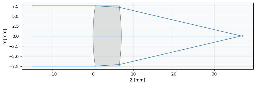
lens = optic.Optic()
lens.surfaces.add(index=0, thickness=be.inf)
lens.surfaces.add(index=1, thickness=7, radius=1000, material="N-SF11", is_stop=True)
lens.surfaces.add(index=2, thickness=30, radius=-1000)
lens.surfaces.add(index=3)
lens.set_aperture(aperture_type="EPD", value=15)
lens.fields.set_type(field_type="angle")
lens.fields.add(y=0)
lens.wavelengths.add(value=0.55, is_primary=True)
_ = lens.draw()

Formulate the Optimization Problem
Here, we define the goal of our optimization. We specify what we want to minimize (the operand) and which parameters we can change (the variables).
[3]:
problem = optimization.OptimizationProblem()
input_data = {
    "optic": lens,
    "surface_number": -1,
    "Hx": 0, "Hy": 0,
    "num_rays": 5,
    "wavelength": 0.55,
    "distribution": "hexapolar",
}
problem.add_operand("rms_spot_size", target=0, weight=1, input_data=input_data)
problem.add_variable(lens, "radius", surface_number=1)
problem.add_variable(lens, "radius", surface_number=2)
Define PyTorch module in Optiland
The OpticalSystemModule wraps our Optiland problem, making it compatible with PyTorch’s ecosystem. This allows us to use standard PyTorch optimizers and training loops.
[4]:
model = OpticalSystemModule(lens, problem)
Define PyTorch Adam Optimizer and pass model parameters
[5]:
optimizer = torch.optim.Adam(model.parameters(), lr=0.1)
Optimize with PyTorch
This is a standard PyTorch training loop. In each step, we calculate the loss (RMS spot size), compute gradients using backpropagation, and update the lens radii with the optimizer.
[6]:
# Store loss values for plotting
losses = []

# Run the optimization for 250 steps
for step in range(250):
    optimizer.zero_grad()       # Reset gradients from the previous step
    loss = model()              # Forward pass: calculate the loss (merit function value)
    loss.backward()             # Backward pass: compute gradients
    optimizer.step()            # Update lens radii based on gradients
    model.apply_bounds()        # (Optional) Apply any defined parameter constraints
    losses.append(loss.item())  # Record the loss for this step
[7]:
# Display optimization problem information
problem.info()
╒════╤════════════════════════╤═══════════════════╕
│    │   Merit Function Value │   Improvement (%) │
╞════╪════════════════════════╪═══════════════════╡
│  0 │             0.00722632 │                 0 │
╘════╧════════════════════════╧═══════════════════╛
╒════╤════════════════╤══════════╤══════════════╤══════════════╤══════════╤═════════╤═════════╤════════════════╕
│    │ Operand Type   │   Target │ Min. Bound   │ Max. Bound   │   Weight │   Value │   Delta │   Contrib. [%] │
╞════╪════════════════╪══════════╪══════════════╪══════════════╪══════════╪═════════╪═════════╪════════════════╡
│  0 │ rms spot size  │        0 │              │              │        1 │   0.085 │   0.085 │            100 │
╘════╧════════════════╧══════════╧══════════════╧══════════════╧══════════╧═════════╧═════════╧════════════════╛
╒════╤═════════════════╤═══════════╤══════════╤══════════════╤══════════════╕
│    │ Variable Type   │   Surface │    Value │ Min. Bound   │ Max. Bound   │
╞════╪═════════════════╪═══════════╪══════════╪══════════════╪══════════════╡
│  0 │ radius          │         1 │  49.3595 │              │              │
│  1 │ radius          │         2 │ -53.7277 │              │              │
╘════╧═════════════════╧═══════════╧══════════╧══════════════╧══════════════╛
[8]:
_ = lens.draw()
Plot Losses
[9]:
plt.plot(losses)
plt.xlabel("Iteration")
plt.ylabel("Loss")
plt.title("Lens Optimization: Spot Size Reduction")
plt.grid(alpha=0.25)
plt.show()
