Tutorial 7b: Differentiable Lens Optimization

Prerequisites: Tutorial 1f (Differentiable Ray Tracing Hello World), Tutorial 5a (Simple Optimization)

Tutorial 1f demonstrated the basics of switching to the PyTorch backend and running a quick gradient-based loop. This tutorial is a deeper dive: we will build a complete differentiable optimization pipeline, compare it to a SciPy baseline, and extend it to multi-field optimization.

By the end you will know how to: - Compute gradients of an optical metric (RMS spot size) with respect to design parameters - Run a PyTorch Adam loop and monitor convergence - Compare differentiable optimization to the Levenberg-Marquardt (LeastSquares) baseline - Optimize a multi-field merit function using autograd - Apply gradient clipping and parameter bounds for stable training

1. Why differentiable optimization?

Traditional merit-function optimizers (Levenberg-Marquardt, Differential Evolution) estimate gradients via finite differences — one extra forward ray-trace per variable. For a 10-variable problem that means 10 extra traces per iteration.

With autograd the gradient arrives essentially free: one forward pass builds the computation graph; .backward() traverses it once to produce exact gradients for all variables simultaneously.

When to use autograd vs. merit-function optimizers:

Situation	Recommendation
Many variables, smooth landscape	Autograd + Adam
Categorical variables (glass choice)	GlassExpert (SciPy)
Non-smooth constraints, global search	Differential Evolution / SHGO
Tight integration with an ML pipeline	Autograd — same graph as the rest of the model

import matplotlib.pyplot as plt
import torch
import torch.optim as optim

import optiland.backend as be

# Switch to the PyTorch backend and enable gradient tracking
be.set_backend("torch")
be.set_device("cpu")
be.set_precision("float64")
be.grad_mode.enable()

print("Backend:", be.get_backend())
print("Precision:", be.get_precision())

Backend: torch
Precision: 64

2. Setting up a differentiable lens

We build a simple singlet. When the PyTorch backend is active, surface parameters (radii, thicknesses) are stored as torch.Tensor objects that participate in the computation graph.

from optiland.materials import Material
from optiland.optic import Optic


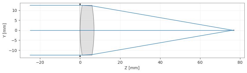
def make_singlet(r1=70.0, r2=-70.0, thickness=70.0):
    """Construct a singlet with the given radii and image distance."""
    lens = Optic(name="Singlet")
    glass = Material("N-BK7")
    lens.surfaces.add(index=0, radius=be.inf, thickness=be.inf)
    lens.surfaces.add(index=1, radius=r1, thickness=7.0, material=glass, is_stop=True)
    lens.surfaces.add(index=2, radius=r2, thickness=thickness)
    lens.surfaces.add(index=3)  # image plane
    lens.set_aperture(aperture_type="EPD", value=25.0)
    lens.fields.set_type("angle")
    lens.fields.add(y=0.0)
    lens.wavelengths.add(value=0.55, is_primary=True)
    return lens


lens = make_singlet()

# The radii are torch tensors with requires_grad=True
r1_param = lens.surfaces.surfaces[1].geometry.radius
r2_param = lens.surfaces.surfaces[2].geometry.radius
print("r1:", r1_param)
print("r2:", r2_param)

r1: tensor(70., dtype=torch.float64, requires_grad=True)
r2: tensor(-70., dtype=torch.float64, requires_grad=True)

3. Computing gradients of an optical metric

We compute the RMS spot radius as a differentiable scalar, then call .backward() to obtain the gradient of the loss with respect to each design parameter.

from optiland.analysis import SpotDiagram


def rms_spot(lens):
    """Return the RMS spot radius as a differentiable scalar tensor."""
    return SpotDiagram(lens).rms_spot_radius()[0][0]


# Zero out any existing gradients
if r1_param.grad is not None:
    r1_param.grad.zero_()
if r2_param.grad is not None:
    r2_param.grad.zero_()

loss = rms_spot(lens)
loss.backward()

print(f"RMS spot radius: {loss.item():.6f} mm")
print(f"d(loss)/d(r1)  : {r1_param.grad.item():.6f}")
print(f"d(loss)/d(r2)  : {r2_param.grad.item():.6f}")

RMS spot radius: 0.944229 mm
d(loss)/d(r1)  : -0.078014
d(loss)/d(r2)  : 0.079865

4. Custom loss function

Any differentiable combination of ray-trace outputs can serve as the loss. Here we define a combined loss that penalises both the RMS spot radius and deviation of the focal length from a target value.

EFL_TARGET = 100.0  # mm


def combined_loss(lens, w_spot=1.0, w_efl=0.1):
    """Penalise RMS spot size + deviation from target focal length."""
    spot = SpotDiagram(lens).rms_spot_radius()[0][0]
    efl = lens.paraxial.f2()
    # Convert to a differentiable scalar tensor
    efl_tensor = be.array(efl) if not isinstance(efl, torch.Tensor) else efl
    efl_penalty = (efl_tensor - EFL_TARGET) ** 2
    return w_spot * spot + w_efl * efl_penalty


loss_val = combined_loss(lens)
print(f"Combined loss: {loss_val.item():.4f}")

Combined loss: 99.0889

5. Full gradient descent optimization loop

We pass the two radius tensors directly to a PyTorch Adam optimizer and run the standard train loop: zero gradients → forward pass → backward → step.

lens = make_singlet()  # fresh lens with default radii
r1_param = lens.surfaces.surfaces[1].geometry.radius
r2_param = lens.surfaces.surfaces[2].geometry.radius

optimizer = optim.Adam([r1_param, r2_param], lr=0.5)

losses = []
n_steps = 150

for step in range(n_steps):
    optimizer.zero_grad()
    loss = rms_spot(lens)
    losses.append(loss.item())
    loss.backward()
    # Clip gradients to prevent instability
    torch.nn.utils.clip_grad_norm_([r1_param, r2_param], max_norm=50.0)
    optimizer.step()

    if (step + 1) % 30 == 0 or step == 0:
        print(f"Step {step+1:3d} | loss={loss.item():.5f} mm "
              f"| r1={r1_param.item():.2f}  r2={r2_param.item():.2f}")

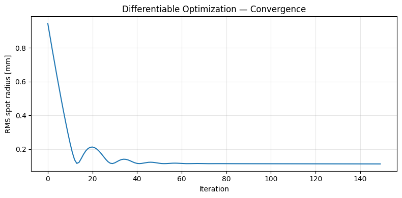
print(f"\nFinal RMS spot: {losses[-1]:.5f} mm")

Step   1 | loss=0.94423 mm | r1=70.50  r2=-70.50
Step  30 | loss=0.11524 mm | r1=76.18  r2=-76.33
Step  60 | loss=0.11655 mm | r1=76.08  r2=-76.67
Step  90 | loss=0.11429 mm | r1=75.90  r2=-77.13
Step 120 | loss=0.11365 mm | r1=75.52  r2=-77.50
Step 150 | loss=0.11299 mm | r1=75.09  r2=-77.94

Final RMS spot: 0.11299 mm

_ = lens.draw()

plt.figure(figsize=(8, 4))
plt.plot(losses)
plt.xlabel("Iteration")
plt.ylabel("RMS spot radius [mm]")
plt.title("Differentiable Optimization — Convergence")
plt.grid(alpha=0.3)
plt.tight_layout()
plt.show()

6. Comparing to the SciPy optimizer

We solve the same problem with Optiland’s LeastSquares optimizer (Levenberg-Marquardt) and compare convergence speed and final result quality.

# Switch back to NumPy for the SciPy baseline
be.set_backend("numpy")

from optiland.optimization import LeastSquares, OptimizationProblem

lens_np = make_singlet()  # re-build under numpy backend

problem = OptimizationProblem()
problem.add_variable(lens_np, "radius", surface_number=1)
problem.add_variable(lens_np, "radius", surface_number=2)
problem.add_operand(
    operand_type="rms_spot_size",
    target=0.0,
    weight=1,
    input_data={
        "optic": lens_np,
        "Hx": 0,
        "Hy": 0,
        "wavelength": 0.55,
        "distribution": "hexapolar",
        "num_rays": 6,  # 6 rings
        "surface_number": -1,  # image surface
    },
)

optimizer = LeastSquares(problem)
result = optimizer.optimize()

np_final_r1 = lens_np.surfaces.surfaces[1].geometry.radius
np_final_r2 = lens_np.surfaces.surfaces[2].geometry.radius
print(f"SciPy LM result: r1={np_final_r1:.4f}  r2={np_final_r2:.4f}")

final_rms = problem.operands[0].value.copy()
print(f"Final RMS Spot Size: {final_rms:.6f} mm")

Warning: Method 'lm' (Levenberg-Marquardt) chosen, but number of residuals (1) is less than number of variables (2). This is not supported by 'lm'. Switching to 'trf' method.
SciPy LM result: r1=76.3238  r2=-76.6639
Final RMS Spot Size: 0.114909 mm

_ = lens_np.draw()

# Restore PyTorch backend
be.set_backend("torch")
be.set_precision("float64")
be.grad_mode.enable()

print(f"Autograd Adam final (r1, r2) : ({r1_param.item():.4f}, {r2_param.item():.4f})")
print(f"\tFinal RMS Spot Size: {losses[-1]:.5f} mm")
print(f"LM (SciPy) final (r1, r2)    : ({np_final_r1:.4f}, {np_final_r2:.4f})")
print(f"\tFinal RMS Spot Size: {final_rms:.6f} mm")

Autograd Adam final (r1, r2) : (75.0938, -77.9356)
        Final RMS Spot Size: 0.11299 mm
LM (SciPy) final (r1, r2)    : (76.3238, -76.6639)
        Final RMS Spot Size: 0.114909 mm

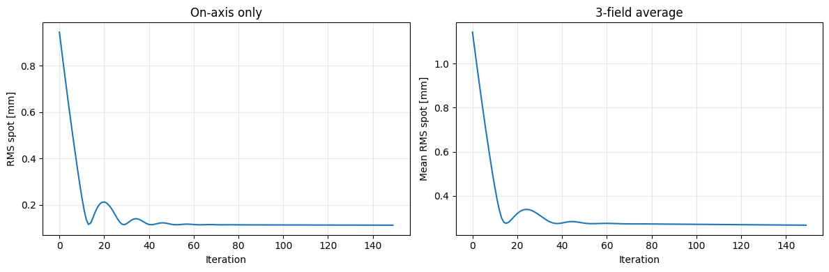
7. Multi-field differentiable optimization

Real designs must perform well across many field points. We build a loss that averages RMS spot size over three normalized field angles and optimize simultaneously.

from optiland.optic import Optic


def make_singlet_multifield(r1=70.0, r2=-70.0, thickness=70.0):
    """Singlet with three field angles."""
    lens = Optic(name="Singlet (multi-field)")
    glass = Material("N-BK7")
    lens.surfaces.add(index=0, radius=be.inf, thickness=be.inf)
    lens.surfaces.add(index=1, radius=r1, thickness=7.0, material=glass, is_stop=True)
    lens.surfaces.add(index=2, radius=r2, thickness=thickness)
    lens.surfaces.add(index=3)
    lens.set_aperture(aperture_type="EPD", value=25.0)
    lens.fields.set_type("angle")
    lens.fields.add(y=0.0)
    lens.fields.add(y=5.0)
    lens.fields.add(y=10.0)
    lens.wavelengths.add(value=0.55, is_primary=True)
    return lens


lens_mf = make_singlet_multifield()
r1_mf = lens_mf.surfaces.surfaces[1].geometry.radius
r2_mf = lens_mf.surfaces.surfaces[2].geometry.radius

optimizer_mf = optim.Adam([r1_mf, r2_mf], lr=0.5)
losses_mf = []

for step in range(150):
    optimizer_mf.zero_grad()
    # Average RMS across all three fields
    rms_all = SpotDiagram(lens_mf).rms_spot_radius()
    loss = sum(rms_all[fi][0] for fi in range(3)) / 3
    losses_mf.append(loss.item())
    loss.backward()
    torch.nn.utils.clip_grad_norm_([r1_mf, r2_mf], max_norm=50.0)
    optimizer_mf.step()

    if (step + 1) % 50 == 0:
        print(f"Step {step+1:3d} | mean RMS={loss.item():.5f} mm "
              f"| r1={r1_mf.item():.2f}  r2={r2_mf.item():.2f}")

Step  50 | mean RMS=0.27707 mm | r1=76.49  r2=-77.46
Step 100 | mean RMS=0.27034 mm | r1=75.66  r2=-78.84
Step 150 | mean RMS=0.26638 mm | r1=74.32  r2=-80.36

fig, axes = plt.subplots(1, 2, figsize=(12, 4))
axes[0].plot(losses)
axes[0].set_title("On-axis only")
axes[0].set_xlabel("Iteration")
axes[0].set_ylabel("RMS spot [mm]")
axes[0].grid(alpha=0.3)
axes[1].plot(losses_mf)
axes[1].set_title("3-field average")
axes[1].set_xlabel("Iteration")
axes[1].set_ylabel("Mean RMS spot [mm]")
axes[1].grid(alpha=0.3)
plt.tight_layout()
plt.show()

8. Practical considerations

Numerical precision: PyTorch defaults to float32. For optical design, switch to float64 (as done in this tutorial) to avoid precision losses in intersection and normal computations.

Parameter bounds: Unconstrained optimizers can walk radii to near-zero (degenerate surfaces). Either clamp with param.data.clamp_(min_val, max_val) after each step, or use Optiland’s TorchAdamOptimizer which handles bounds automatically.

Gradient clipping: Large gradients (especially early in training) can cause NaN. Clip with torch.nn.utils.clip_grad_norm_ as shown above.

When to use Optiland’s built-in PyTorch optimizer: For standard workflows, TorchAdamOptimizer (via OptimizationProblem) handles gradient enabling, parameter wrapping, bounds, and scheduling automatically:

from optiland.optimization import OptimizationProblem, TorchAdamOptimizer

problem = OptimizationProblem()
problem.add_variable(lens, 'radius', surface_number=1)
problem.add_variable(lens, 'radius', surface_number=2)
problem.add_operand('rms_spot_size', target=0.0, weight=1,
                    input_data={'optic': lens, 'Hx': 0, "Hy": 0,
                                'wavelength': 0.55, 'distribution': 'hexapolar',
                                'num_rays': 6, "surface_number": -1})

opt = TorchAdamOptimizer(problem)
opt.optimize(n_steps=200, lr=0.5)

Use the manual loop (as in this tutorial) when you need a custom loss function, gradient clipping, multi-task loss weighting, or integration with an external ML training loop.

Conclusion

In this tutorial you learned how to:

• Enable the PyTorch backend and compute gradients of optical metrics

• Run a standard Adam loop with gradient clipping for stable convergence

• Define a custom combined loss (spot size + focal length penalty)

• Compare autograd optimization to a SciPy Levenberg-Marquardt baseline

• Extend to multi-field optimization with a single .backward() call

Next steps: - Try optimizing conic constants or freeform coefficients in addition to radii - Use GPU acceleration with be.set_device('cuda') for large ray sets - Integrate the differentiable lens into a larger PyTorch model for end-to-end camera-system training