Tutorial 6c: Roughness, Scattering and Extended Sources

Consolidating micro-roughness, BSDF scattering propagation, and extended source modeling.

This tutorial demonstrates how surface roughness and scattering can be configured on surfaces in Optiland. We will compare singlets with the following scattering properties assigned:

• No scattering

• Gaussian Scattering

• Lambertian Scattering

The scattering model is defined via the Bidirectional Scattering Distribution Function, or BSDF.

import matplotlib.pyplot as plt
import numpy as np

from optiland import optic, scatter

Preparation

We first define a generic singlet class that accepts a bsdf as an input. In this example, we assign the scattering only to the rear surface.

class SingletConfigurable(optic.Optic):
    def __init__(self, bsdf):
        super().__init__()

        # add surfaces
        self.surfaces.add(index=0, radius=np.inf, thickness=np.inf)
        self.surfaces.add(
            index=1,
            thickness=7,
            radius=50,
            is_stop=True,
            material="N-SF11",
        )
        self.surfaces.add(index=2, thickness=50, bsdf=bsdf)  # <-- add bsdf here
        self.surfaces.add(index=3)

        # add aperture
        self.set_aperture(aperture_type="EPD", value=25.4)

        # add field
        self.fields.set_type(field_type="angle")
        self.fields.add(y=0)
        self.fields.add(y=10)
        self.fields.add(y=14)

        # add wavelength
        self.wavelengths.add(value=0.48613270)
        self.wavelengths.add(value=0.58756180, is_primary=True)
        self.wavelengths.add(value=0.65627250)

        self.image_solve()  # solve for image plane

Let’s also define a helper function to plot a 2D distribution of rays intersection points.

def plot_ray_distribution(rays, bins=128):
    x = rays.x
    y = rays.y
    i = rays.i

    plt.hist2d(x, y, weights=i, bins=bins, cmap="viridis")
    plt.colorbar()
    plt.xlabel("X (mm)")
    plt.ylabel("Y (mm)")
    plt.title("2D Ray Distribution on Image Plane")
    plt.show()

1. Singlet #1 - No Surface Scattering

The first singlet we analyze will have no scattering applied. Let’s first define the lens and draw it.

singlet_no_scatter = SingletConfigurable(bsdf=None)

singlet_no_scatter.draw()

Let’s trace 1 million random rays through the lens at the on-axis field point and look at the distribution.

rays = singlet_no_scatter.trace(
    Hx=0,
    Hy=0,
    wavelength=0.58756180,
    num_rays=1_000_000,
    distribution="random",
)

plot_ray_distribution(rays, bins=128)

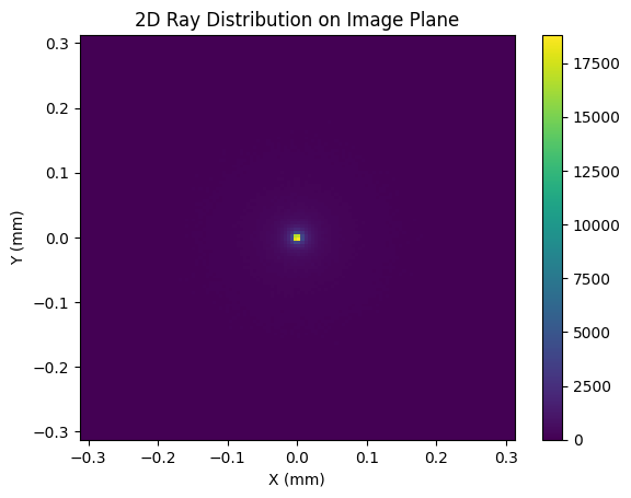
As we can see, the energy is largely located at the origin on the image plane. Let’s see how this is implacted when scattering is introduced.

2. Singlet #2 - Gaussian Scattering

Gaussian scattering is defined by a 2D Gaussian distribution with a user-defined sigma (std. dev.) value. The larger the value of sigma, the closer the scattering model comes to Lambertian. We define a GaussianBSDF model with a sigma value of 0.01 and generate a new singlet:

bsdf = scatter.GaussianBSDF(sigma=0.01)
singlet_gaussian = SingletConfigurable(bsdf=bsdf)

Again, we trace 1 million rays and view the distribution at the image plane:

rays = singlet_gaussian.trace(
    Hx=0,
    Hy=0,
    wavelength=0.58756180,
    num_rays=1_000_000,
    distribution="random",
)

plot_ray_distribution(rays)

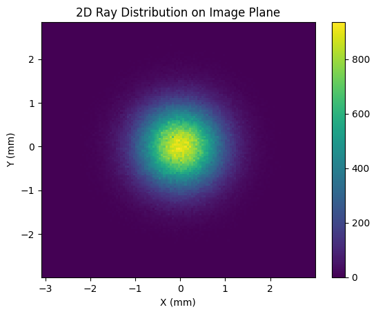
The image size has blurred significantly in comparison to the no-scattering case. Note that the plot axis spans a larger range here as well.

3. Singlet #3 - Lambertian Scattering

Lambertian scattering implies that the surface scatters incident light uniformly in all directions. Diffuse surfaces can be considered approximately Lambertian. To model a Lambertian scatterer in Optiland, we simply define the LambertianBSDF model and pass it to our singlet:

bsdf = scatter.LambertianBSDF()
singlet_lambertian = SingletConfigurable(bsdf=bsdf)

rays = singlet_lambertian.trace(
    Hx=0,
    Hy=0,
    wavelength=0.58756180,
    num_rays=1_000_000,
    distribution="random",
)

plot_ray_distribution(rays, bins=np.linspace(-100, 100, 128))

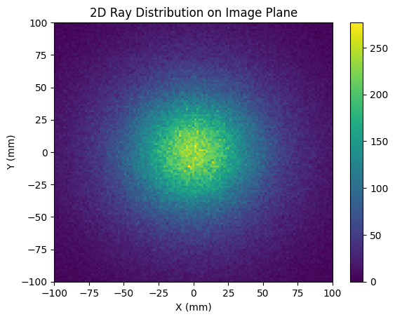
In this case, we are plotting the image plane over a significantly larger area, from -100 mm to 100 mm. Clearly, the Lambertian scatter model has dramatically increased the spot size at the image plane.

4. Conclusions:

• We introduced two BSDF scatter models: Gaussian and Lambertian.

• Scatter models can be used to model and understand the impact of manufacturing defects, such as surface roughness on optical surfaces.

---

Part 2: Extended Source Modeling

import optiland.backend as be
from optiland.optic import Optic, ExtendedSourceOptic
from optiland.sources import SMFSource
from optiland.analysis import IncoherentIrradiance
from optiland.physical_apertures import RectangularAperture

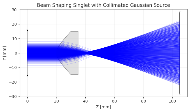
1. Define the Optical System

First, we define the Beam Shaping Singlet system. This system is designed to transform a Gaussian beam into a flat-top profile.

gaussian_beam_waist = 5.0  # in mm
wavelength_um = 0.55  # in µm

# Forbes QBFS surface parameters
forbes_terms = {
    0: 0.5414,
    1: 0.6689,
    2: 0.3409,
    3: -0.0537,
    4: -0.3960,
    5: -0.2991,
    6: 0.3921,
}
forbes_norm_radius = 30.3636
top_hat_radius = 25.0

# Create the Optic
lens = Optic()
lens.set_aperture(
    aperture_type="EPD", value=gaussian_beam_waist * 6
)
lens.wavelengths.add(value=wavelength_um, is_primary=True)
lens.fields.set_type(field_type="angle")
lens.fields.add(y=0.0)

# Add surfaces
lens.surfaces.add(index=0, thickness=be.inf)
lens.surfaces.add(
    index=1,
    thickness=20.0,
    is_stop=True,
    aperture=RectangularAperture(
        x_min=-15,
        x_max=15,
        y_min=-15,
        y_max=15,
    ),
)
lens.surfaces.add(
    index=2,
    surface_type="forbes_qbfs",
    radius=5.7410,
    conic=-2.3165,
    thickness=15.0,
    material="N-BK7",
    radial_terms=forbes_terms,
    norm_radius=forbes_norm_radius,
    aperture=30.0,
)
lens.surfaces.add(
    index=3,
    surface_type="standard",
    radius=be.inf,
    thickness=70.0,
    material="air"
)
lens.surfaces.add(
    index=4,
    aperture=RectangularAperture(
        x_min=-top_hat_radius * 1.1,
        x_max=top_hat_radius * 1.1,
        y_min=-top_hat_radius * 1.1,
        y_max=top_hat_radius * 1.1,
    ),
)

Note on Normalization Radius (``norm_radius``):

In optiland, when you explicitly provide normalization parameters (like norm_radius for Forbes/Zernike surfaces, or norm_x/norm_y for Chebyshev surfaces) during geometry initialization, the surface’s normalization_mode is automatically set to 'manual'.

This means the radius is locked to your provided value and will not be automatically scaled during paraxial updates. If you omit the normalization parameters, the normalization_mode defaults to 'auto', and the normalization radius will dynamically scale to \(1.25 \times \text{semi-aperture}\).

2. Setup Extended Source

We use SMFSource to represent a collimated Gaussian source.

Note on Collimation: To approximate a collimated source using SMFSource, we set the divergence angle to an extremely small value (e.g., 1e-10 degrees). The Mode Field Diameter (MFD) determines the spatial extent of the beam. Here we set it to \(2 × \text{waist} = 10\text{ mm} = 10000\text{ µm}\).

# MFD is in microns. 2 * waist (5mm) = 10mm = 10000um
mfd_microns = gaussian_beam_waist * 2 * 1000

# Create the source
source = SMFSource(
    mfd_um=mfd_microns,
    wavelength_um=wavelength_um,
    divergence_deg_1e2=1e-10,  # Virtually zero divergence for collimation
    total_power=1.0,
    position=(0, 0, 0)
)

# Wrap the optic with the source
ext_optic = ExtendedSourceOptic(lens, source)

print(source)

SMFSource(mfd=10000.0µm, divergence=1e-10°, wavelength=0.55µm, power=1.0W, mode=extended, position=(0.0, 0.0, 0.0))

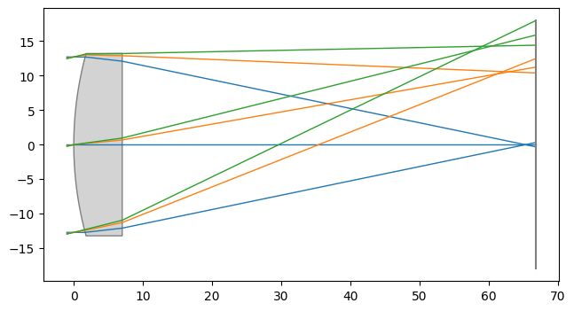
3. Visualization

We can now draw the optical system with the source rays traced through it. The draw method of ExtendedSourceOptic handles this automatically.

fig, ax = ext_optic.draw(num_rays=1000, title="Beam Shaping Singlet with Collimated Gaussian Source")
fig.show()

C:\Users\kdani\AppData\Local\Temp\ipykernel_1988\284778195.py:2: UserWarning: FigureCanvasAgg is non-interactive, and thus cannot be shown
  fig.show()

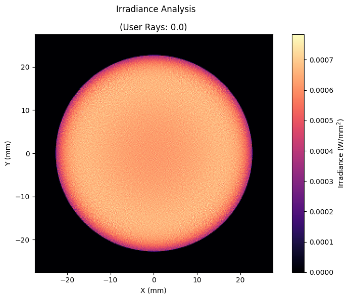
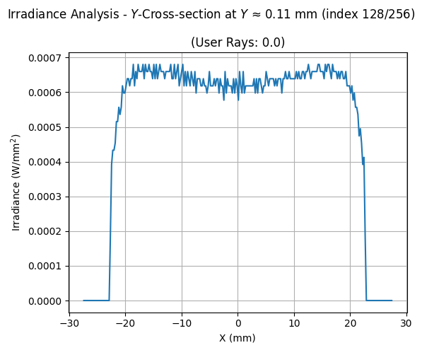
4. Irradiance Analysis

Finally, we calculate and visualize the irradiance at the image plane. We trace a larger number of rays for better resolution and use IncoherentIrradiance.

# Compute and plot irradiance
analysis = IncoherentIrradiance(lens, source=source, num_rays=1_000_000, detector_surface=-1, res=(256, 256))
analysis.view(figsize=(8, 6), cmap="magma", normalize=False)
analysis.view(cross_section=("cross-y", 128), normalize=False)

(<Figure size 600x500 with 1 Axes>,
 array([[<Axes: title={'center': '(User Rays: 0.0)'}, xlabel='X (mm)', ylabel='Irradiance (W/mm$^2$)'>]],
       dtype=object))